Diffusion Models (DRAFT)

The overarching goal of diffusion models is to predict the noise that was added to an image at any time between $t-1$ and $t$.

We want to add noise to the image such that the noisy image at $X_t$ is Gaussian, i.e. ${N}(0, 1)$, which is required to create a learnable loss function and because standard Gaussians give us nice mathematical properties and, thus, are easy to work with.

Noise is added gradually, instead of one large addition of Gaussian noise. Just a bit in the beginning, then more towards the end when the image is almost fully Gaussian anyway. We do this, because we want to learn to undo the noise that was added between step $t$ and $t-1$.

The reasoning is that it’s easier to learn to undo a bit of noise, rather than a lot of noise across many time steps.

Forward Process

In order to get the noisy images to train, we need to generate them. This is naive, flawed approach:

Here, $\epsilon_t$ is the Gaussian noise added at time $t$.

The $\beta$ term is added to scale down the Gaussian noise. This is required, because the input images are often normalised, usually between 0 and 1. Standard Gaussian noise can return numbers like $0.8$, which will quickly overwhelm the numbers of the input image. Therefore, the Gaussian noise needs to be scaled down.

With this current setup, we need to have the previous noisy image $X_{t-1}$ to generate the next noisy image $X_t$. But we can rewrite this to get any $X_t$ just from the starting image $X_0$. E.g.:

If you have zero mean, scaled Gaussians, you can sum the variances, which gives you a “new” Gaussian:

But unfortunately, $X_t = N(X_0, t\beta) \neq N(0,1)$ because $X_0 \neq 0$ and $t\beta \neq 1$.

We can even see this visually if we add the noise to an image in this iterative way and compare this to what standard Gaussian noise would look like.

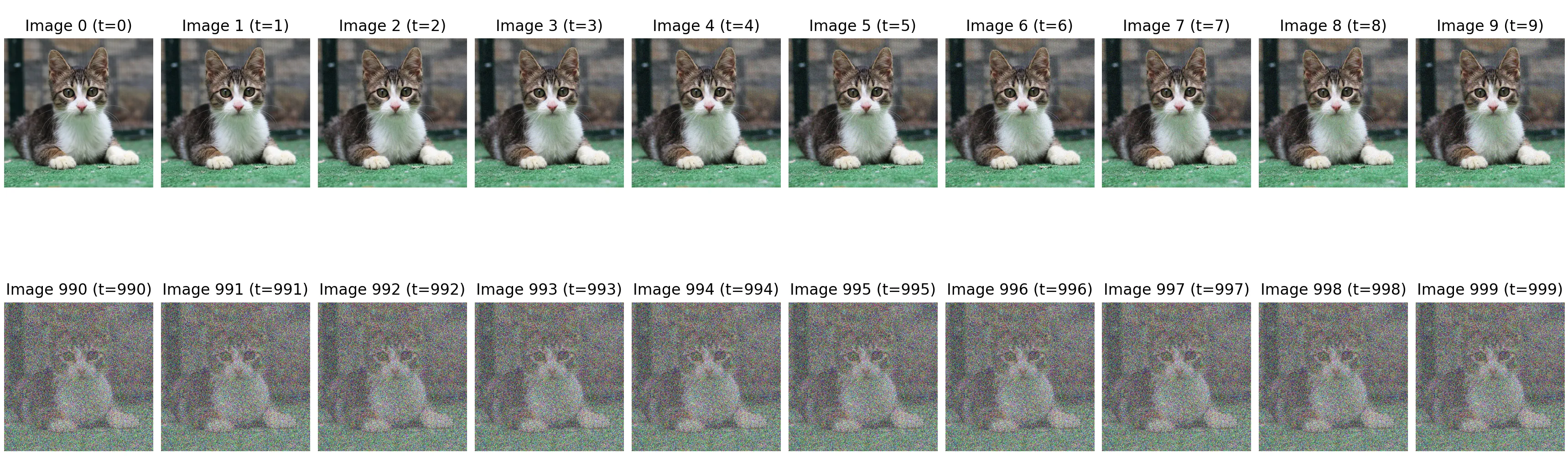
This is what the iterative approach would look like (which also takes a lot of time to run). Using the direct approach, we can get the final noisy image faster:

But as can be seen, the noisy image looks much different that what true Gaussian noise would look like. This further shows that our naive approach does not converge to a standard Gaussian.

A better approach is needed. The authors came up with this formula:

where $\beta_t$ is the scalar at time step $t$ (following a schedule e.g.). However, the issue still persists that we need to compute $X_{t-1}$ to compute $X_t$. But we’d much rather have a function that takes the initial $X_0$ and $t$ as input at outputs the correct $X_t$ directly. Let’s have a look at what $X_{t-1}$ looks like.

If we substitute $X_{t-1}$ into the $X_t$ equation, we get

Now, we say that $\alpha_t = 1 - \beta_t$ to make this easier to read and have less clutter:

Now we can re-use our neat trick from before where we said that variances of zero-mean Gaussians ($\epsilon_{t-1}$ and $\epsilon_t$ in our case) can be summed up. Remember, that in this equation we are working with standard deviations (i.e. $\sigma$) but variances are the squares of standard deviations (i.e. $\sigma^2$). This means, we need to square our standard deviations to get the variance first, i.e.:

The variance of a Gaussian is 1, which gives us:

This means that if we sum up the variances, we get a new Gaussian with mean 0 and variance $1-\alpha_t\alpha_{t-1}$. In other words:

I denoted the new Gaussian noise as $\epsilon'$. From here, we can notice a pattern! We managed to describe $X_t$ as a combination from the noisy image two steps before and this has added another $\alpha$ term into the square roots. If we repeat this process until we get to $X_0$, we have this:

We can simplify this a bit further by saying $\bar\alpha_t = \prod_i^t \alpha_t$, which gives us our final statement:

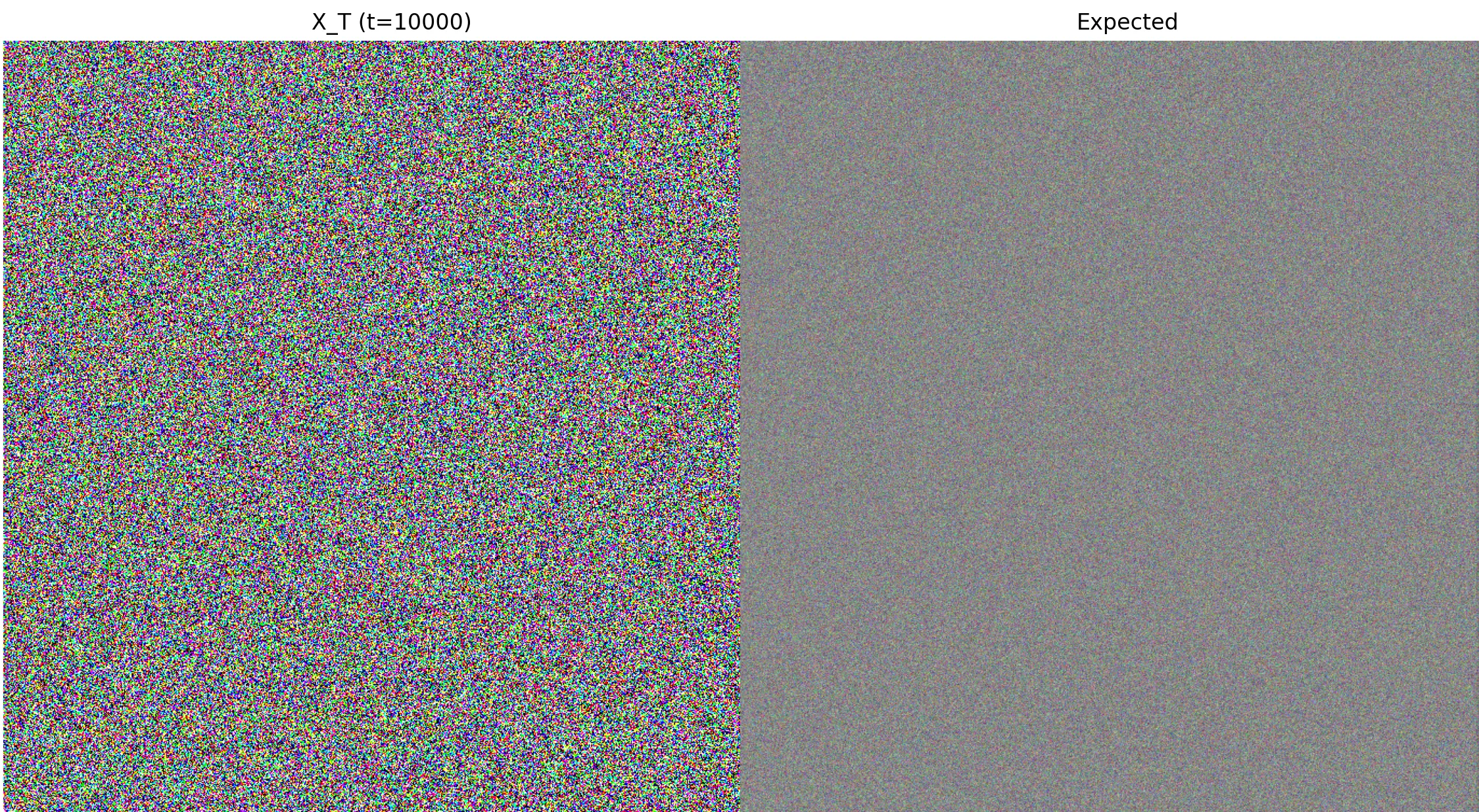
And there we go! Now we can generate the final noisy image at time step $t$ just by having the initial image $X_0$. Using this new formula, we can compare the generated noisy image from what we had generated before:

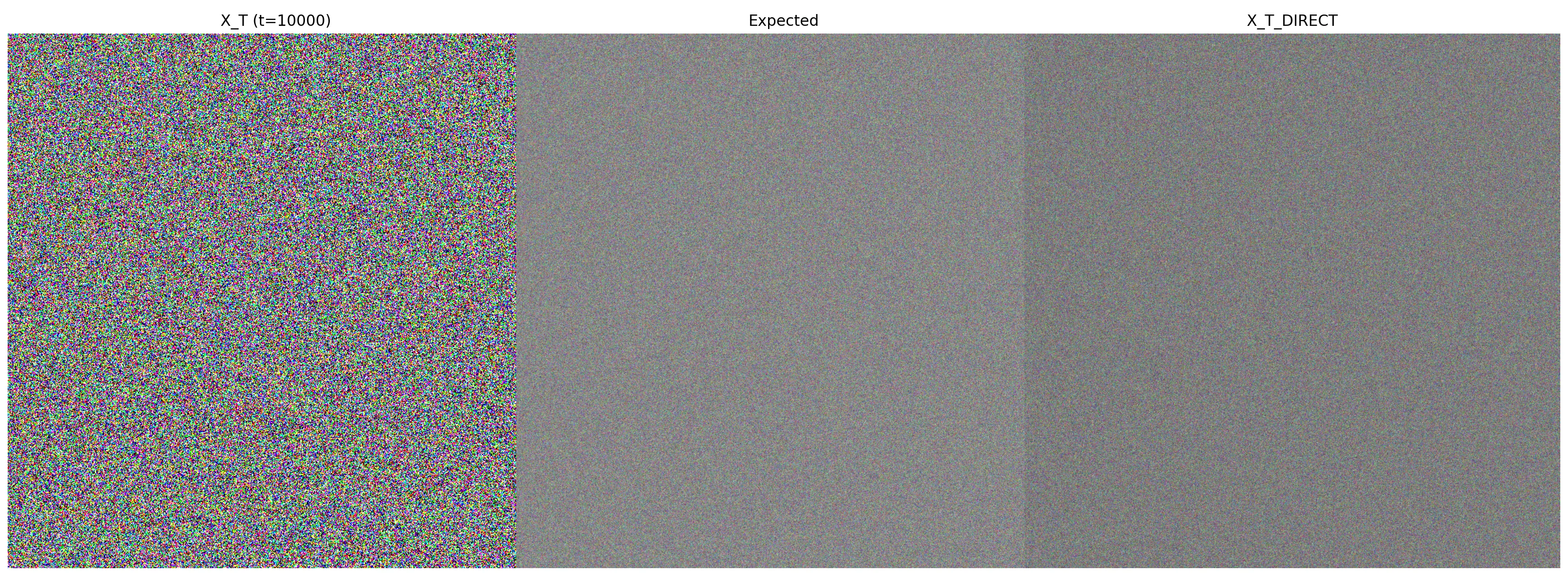
Now this looks much closer to Gaussian noise than what we had before. It’s a bit darker due to the larger value for $\beta$ that I used. However, mathematically, this does converge to a standard Gaussian

Because as we increase $t$, we keep multiplying more and more numbers that are between 0 and 1 (because remember that $\beta$ needs to be in that range), thus making the square root smaller and smaller, which in the limit becomes 0 and $0 X_0 = 0$. Similarly, as time goes on and $\bar{\alpha_t}$ moves towards 0, the square root converges towards 1, which then just adds regular Gaussian noise via $\epsilon'$.

With this, we have the forward method covered. Now it’s time to derive the loss function and the learning objective.

Deriving the Loss Function

So far, we have described the forward process as a step-by-step sampling procedure. This is great for building intuition. However, to create a loss function, we need to shift from the language of single samples ($X_t$) to the language of probability distributions. This is important, because as we try to predict the noise added at a particular step $X_t$, we don’t actually know exactly what noise has to be added in general. Think of it this way:

You have some $X_t$ and sample some noise to get $\epsilon_t$, you add that in and then get $X_{t+1}$. But this amount of noise and this specific $X_t$ are just some samples. There are many more $X_t$ and $\epsilon_t$ that could result in $X_{t+1}$, it’s like a whole cloud. These specific values might have come from the edge of the cloud. If you just computed the MSE from that, you wouldn’t learn the true average, which you would find in the center of the cloud. By thinking about this as a probability distribution, you need to find the loss between your model and the center of the cloud.

The formal name for the distribution defined by our single-step sampling process is $q(X_t|X_{t-1})$.

The Markov Chain Property

A crucial property of our forward process is that it’s a Markov Chain. This simply means that the distribution for the next state, $X_t$, depends only on the immediately preceding state, $X_{t-1}$. It does not depend on any other previous states like $X_{t-2}$, $X_{t-3}$, or the original $X_0$.

The Joint Probability Distribution

We want to find the probability of an entire sequence of noisy images, $X_1, \dots, X_T$, given our starting image $X_0$. This is the joint probability distribution, $q(X_{1:T}|X_0)$.

Using the general chain rule of probability, we would write this as: $q(X_1, \dots, X_T | X_0) = q(X_1 | X_0) \cdot q(X_2 | X_1, X_0) \cdot \dots \cdot q(X_T | X_{T-1}, \dots, X_0)$ This looks complicated because each step seems to depend on the entire history.

However, we can now apply our Markov assumption. The assumption that $X_t$ only depends on $X_{t-1}$ allows us to simplify each term:

• $q(X_2 | X_1, X_0)$ simplifies to just $q(X_2 | X_1)$.
• $q(X_T | X_{T-1}, \dots, X_0)$ simplifies to just $q(X_T | X_{T-1})$. Applying this simplification across the entire chain gives us a much cleaner result: $q(X_1, \dots, X_T | X_0) = q(X_1 | X_0) \cdot q(X_2 | X_1) \cdot \dots \cdot q(X_T | X_{T-1})$Finally, we can write this long product in a compact form using the product symbol, $\prod$: $q(X_{1:T} | X_0) = \prod_{t=1}^{T} q(X_t | X_{t-1})$ This final equation is the formal definition of our entire forward process.

For the reverse process, we have our model $p_\theta$. To get a clean image back, we have to compute the joint probability, i.e.:

From here we can start with the loss function derivation, because as stated before, we want to sample a clean image using our model. To do that, we need to minimise the negative log likelihood:

If we can minimise this, then we are learning the true data distribution, i.e. our dataset.

From here the first step is marginalisation using the Chain Rule of Probability:

This loss function is numerically intractable, because we can’t integrate over all possible $X$ in existence. We need to insert something into this intractable integral to make it tractable. We can use the “divide-by-one” trick (I’m not sure if that’s what it’s called - I just like to call it that):

Now, this is in the form of an expectation, i.e.:

Therefore, if we rewrite this into the form of an expectation, we get

I did this definition:

just so the math is a bit more concise.

Now we need to apply the logarithm:

Because $\log$ is a concave function, we can apply Jensen’s Inequality, which states:

This gives us:

Now we have a lower bound. If we can make the expectation smaller, we will also minimise the negative log likelihood, which is exactly what we want. Thus, our new loss function to minimise is

We can apply this log rule to get rid of the negative sign $\log(A/B)=−\log(B/A)$.

Now, we can use this log rule $\log(A/B)=\log A−\log B$

Because $\log(A⋅B)=\log A+\log B$, we can turn the products into sums and remove the brackets of the left log part:

You will also notice that I separated the $t=1$ step. This is required in order to apply Bayes’ rule.

But if you instead did this:

You would get a so-called Dirac Delta function $p(a|a)=\delta(0)$, which is a point mass “probability distribution” which in turn isn’t really a probability distribution, because there is no uncertainty. It’s like saying “What card do I hold on my hand given that I hold the ace of hearts?”. It’s a tautology. This means you can’t apply Bayes’ rule here in a matter that makes sense, therefore you exclude this part.

Now we can rewrite the fraction in the sum using Bayes’ Rule (and the log rule where a product becomes a sum).

What we have now is a so called telescoping sum, which comes from this part:

If you were to write out the terms you would get something like this (I will simplify this to just tuples, assume that the tuple (0,0) is equal to one, because $\log(q|q)=\log(1)=0$):

The tuples being placeholders, e.g. $(1,0) \equiv \log q(X_1|X_0)$ or $(2,1) \equiv \log q(X_2|X_1)$ etc. As you can see, all the pairs cancel out except for the last one. This simplifies the sum to be this:

Ok, so now we have 3 terms and whenever you see a log of a quotient, you have to think “KL Divergence”, which measures the distance between two probability distributions, i.e.:

Or for continuous probabilities:

Or if written in the form of an expectation:

This is exactly what we have in our loss term:

If we have a closer look, we can see that the left KL divergence has no trainable parameters $\theta$ in it, so we can safely ignore it, as it will become 0 as soon as we compute the gradient. As for the rightmost part, the authors of the DDPM paper have seen that, empirically, it makes no difference to leave that part it, so we can also leave that part out. This leaves us with this:

The good thing is that if your probability distributions are Gaussian, they simplify to a nice closed form. In general, for two univariate Gaussians, you have

and for multivariate Gaussians, you have this:

In the above formula, $|\Sigma|$ is the determinant, $d$ is the dimensionality and $\text{tr}$ is the trace. Crucially, the authors set the covariances (variances) of both Gaussians to be equal, which means their determinants are also equal, which means two things:

First:

And second:

And therefore, you have this $0−d+d=0$, which means that only the means survive:

Because we set the variance to a constant, $\Sigma^{-1}$ is just a constant factor, which plays no role when we minimise the loss function, so we can leave it out, which finally brings us to this part:

There is one last step, which is the reparameterisation trick. This was our forward step:

Which we can solve for $X_0$

The true posterior mean has this form:

If we substitute $X_0$, we get:

Doing a bit of algebra and collecting the $X_t$ terms, we arrive at:

In this form, the true mean is now expressed as a combination of $X_t$ and the true noise $\epsilon$. If we now change our neural network to output not the mean, but rather the noise directly, we get this:

If we insert this into the above loss expression, we get this:

Which finally brings us to