Graph Neural Netwroks - Quickstart

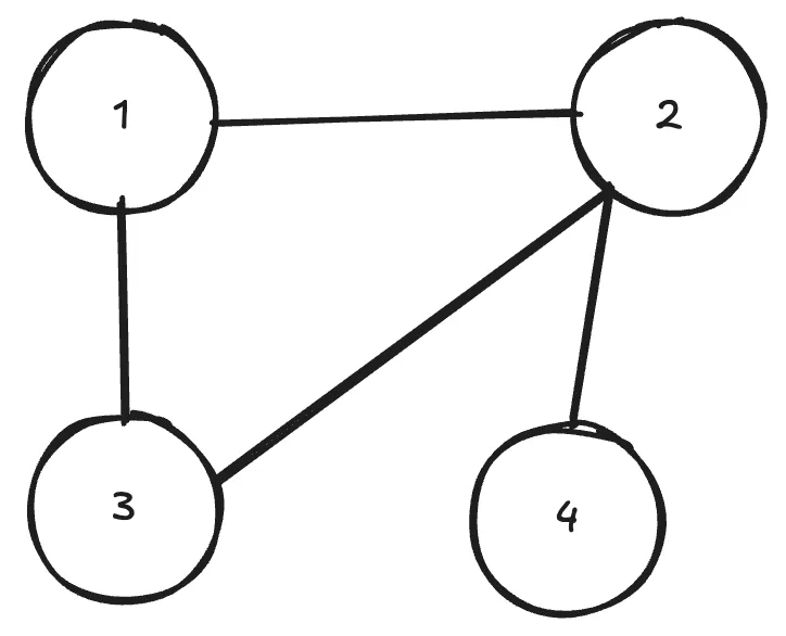
Many things in life can be represented easily as graphs. One classical example would be a social network, where nodes are people and edges between the nodes represent some kind of connection, like friendship for example. Here’s a simple example of a graph.

GNNs allow us to make some kind of prediction on the whole graph or parts of it. E.g. if the whole graph was a molecule, you could try to predict chemical properties of it. You could also predict a missing connection (edge) between some nodes. Lots of interesting things!

How do we represent a graph like this in order to feed this to our neural network? First, lets think of the features of each node using our example of molecules. Each node (atom) could have several properties, such as atomic weight, number of neutrons etc. We simply denote the number of features per node as $n$ and the number of total nodes as $m$. If we were to list them in a matrix, it would have the shape $m\times n$, i.e. $m$ nodes, each with $n$ features. We could feed this directly into our neural network (nothing in the universe stops us from doing this), but we’d be missing the most crucial aspect, which makes a neural network a graph neural network, namely the neighbours.

A simple $m\times n$ matrix doesn’t capture the information that node 1 is connected to node 3 and 2. So how do we include this information? To do that, we need to represent somehow which node is connected to which other node. This is called an adjacency matrix. If there is a connection between the nodes, the value is 1, else 0. For the example above, the adjacency matrix looks like this $m\times m$ matrix:

Note that we put $1$s on the diagonal. This effectively means every node is connected to itself, so it remembers its own information during the update.

Ok, now we know which node is connected to which other node and each of the features of our nodes. To summarise the shapes, we have an $m\times n$ matrix which hosts the features of our nodes (which we will call $F$ from now on) and an $m\times m$ adjacency matrix (called $A$). But we can’t just do $A \times F$ and call it a day. Think about what $A\times F$ means. You take the rows of $A$ and multiply by the columns of $F$. Let me introduce a concrete example with some made up numbers:

Each column of $F$ represents the first feature value of every node, and each row of $A$ tells you to which nodes that node is connected to. Lets look at the first row of $A$ and first column of $F$:

When we multiply these element-wise and then take the sum, we get the value of the solution matrix at position $0,0$ (i.e. the top left value). In this case, the solution is $1 * 0 + 1 * 1.0 + 1 * 1.0 + 0 * 1.5 = 2.0$. But this is kind of flawed. What if our first node had 1000 neighbours, and the second node had only 1? In this case, the value for the first node would be MUCH bigger than for the second one and further along the network it might just get bigger and bigger, leading to a gradient explosion later on. The solution to this problem is to normalise the adjacency matrix by their degree. This sounds complicated, but really isn’t. All you need to do is to divide $A$ by the sum along the second axis. E.g.:

One thing to note is that our $A$ matrix has ones along its main diagonal, therefore $d$ can’t have $0$ in it. But this is not always the case, especially if not all graphs have the same number of nodes. In that case you add “ghost” nodes (kind of like a padding). Those don’t have neighbours and should be disregarded throughout the neural network, therefore we can’t have THOSE also have a $1$ in the diagonal. But, to make sure that we don’t divide by $0$, we would usually do something like this

degree = jnp.sum(adj, axis=1, keepdims=True)

safe_degree = jnp.where(degree == 0, 1.0, degree)
norm_adj = adj / safe_degree

Let’s think about what this normalisation actually did. Instead of taking the whole feature value of a neighbour node, we just take a little bit of it instead and we do that for every neighbour value. Now, when we aggregate our nodes, like this

aggs = norm_adj @ nodes

then each node in the aggs matrix (of shape $m\times n$) also contains some information about its neighbours as well.

(Note that we haven’t done any learning yet, so far we just averaged. We can now take this aggs matrix and pass it to a linear layer to have some trainable parameters)

Concretely for the first node and the first value, we had before this:

But if we normalise, we get this:

Multiply and take the sum, the total is $~0.67$. This number contains the information from the original node ($0.0$), a bit of the first feature of node 2 ($0.33 * 1.0$), a bit of node 3 ($0.33*1.0$) and none of node 4 ($0.0 * 1.5$) because it is not connected to that node 4. In a way, we collected the information of the neighbours of node 1 and put it all together into this single number. And by the way, this is also the reason, why this type of GNN is called a convolutional GNN, because we computed the convolution between our node and its neighbours using a fixed ‘averaging’ kernel defined by the graph structure.

Okay, enough theory, let’s start with some code. And for this exercise we will use deepchem, a library containing lots of exercises and datasets for you to begin your journey into computational biology.

First, we import our usual suspects:

import typing

import deepchem as dc
import equinox as eqx
import jax
import jax.numpy as jnp
import optax
from deepchem.data import DiskDataset
from deepchem.models.graph_models import ConvMol
from jaxtyping import Array, Float, Int, PRNGKeyArray, PyTree

And now we can explore our data a bit.

tasks, datasets, transformers = dc.molnet.load_tox21(featurizer="GraphConv")
print(tasks)


train_dataset, valid_dataset, test_dataset = datasets
train_dataset = typing.cast(DiskDataset, train_dataset)
valid_dataset = typing.cast(DiskDataset, valid_dataset)
test_dataset = typing.cast(DiskDataset, test_dataset)

first = train_dataset.X[0]
print(train_dataset.y.shape)
first = typing.cast(ConvMol, first)
print(first.get_adjacency_list())
print(first.get_atom_features().shape)

Let’s have a look at the output:

['NR-AR', 'NR-AR-LBD', 'NR-AhR', 'NR-Aromatase', 'NR-ER', 'NR-ER-LBD', 'NR-PPAR-gamma', 'SR-ARE', 'SR-ATAD5', 'SR-HSE', 'SR-MMP', 'SR-p53']
(6258, 12)
[0. 0. 0. 0. 0. 0. 0. 0. 0. 0. 0. 0.]
[[9], [10], [10], [8], [8], [10], [9], [8], [9, 3, 4, 7], [0, 6, 8, 10], [9, 1, 2, 5]]
(11, 75)

We can see that there are 12 tasks for this database. These are so called assays for the tox21 dataset. An assay is simply a test that measures whether something happens. E.g. you put some cells on a test plate, add some chemical and see what happens to the cell. In this case, we have binary outputs, so it could mean that the added chemical activated the biological target (which can be a cell or protein, etc.).

Furthermore, we can see that we have 6258 training points, and that this specific molecule has 11 atoms, each having 75 features. But this doesn’t always need to be the case, the next atom could have 20 or even 120. So we need to set a MAX_ATOMS value that we are sure is greater than all the molecudes in our dataset and “pad” the molecules with these “ghost atoms” (which I mentioned before). This is required specifically for JAX, because in JAX-land, you mustn’t have dynamic length inputs. We’ll set MAX_ATOMS = 150 which should be enough.

We have to do a bit more work on the data, before we can get to the actual models. I’ll show you the code first and then describe what’s going in there:

def collate_batch(
    batch_of_mols: list[ConvMol], in_size: int, max_atoms: int
) -> tuple[
    Float[Array, "batch_size max_atoms in_size"],
    Float[Array, "batch_size max_atoms max_atoms"],
    Float[Array, "batch_size max_atoms 1"],
]:
    batch_size = len(batch_of_mols)

    batch_nodes = jnp.zeros((batch_size, max_atoms, in_size))
    batch_adj = jnp.zeros((batch_size, max_atoms, max_atoms))
    batch_mask = jnp.zeros((batch_size, max_atoms))

    for i, mol in enumerate(batch_of_mols):
        n_atoms = mol.get_num_atoms()
        batch_nodes = batch_nodes.at[i, :n_atoms].set(mol.get_atom_features())

        adj_matrix = jnp.zeros(shape=(max_atoms, max_atoms))
        for j, atom in enumerate(mol.get_adjacency_list()):
            adj_matrix = adj_matrix.at[j, atom].set(1)

        A_tilde = adj_matrix + jnp.zeros_like(adj_matrix).at[:n_atoms, :n_atoms].set(
            jnp.identity(n_atoms)
        )
        batch_adj = batch_adj.at[i].set(A_tilde)

        batch_mask = batch_mask.at[i].set(
            jnp.concat((jnp.ones(shape=(n_atoms)), jnp.zeros(max_atoms - n_atoms)))
        )
    batch_mask = jnp.expand_dims(batch_mask, axis=-1)

    return batch_nodes, batch_adj, batch_mask

Ok, let’s have a look at the first part:

def collate_batch(
    batch_of_mols: list[ConvMol], in_size: int, max_atoms: int
) -> tuple[
    Float[Array, "batch_size max_atoms in_size"],
    Float[Array, "batch_size max_atoms max_atoms"],
    Float[Array, "batch_size max_atoms 1"],
]:
    batch_size = len(batch_of_mols)

    batch_nodes = jnp.zeros((batch_size, max_atoms, in_size))
    batch_adj = jnp.zeros((batch_size, max_atoms, max_atoms))
    batch_mask = jnp.zeros((batch_size, max_atoms))

This should be the simplest part. We get as input a batch of ConvMol which is the specific class in deepchem. The parameter in_size isn’t actually strictly needed and we could infer it from the batch_of_mols, but it basically tells us how many features per atom there are (in this example its $75$) and max_atoms we just discussed earlier. We then create the 3 batch matrices that our model will get as input.

But hold on, what’s this batch_mask? We didn’t cover that one yet, but it’s purpose is to mask out all the ghost atoms that we pad later (e.g. when we use the linear layer or an activation function¹). Basically, when our GNN layer returns something, the parts that we added as ghost atoms must be 0 in the returned matrix, otherwise they would have “meaning” (but they shouldn’t). So whatever we return, we multiply in the end by this mask.

for i, mol in enumerate(batch_of_mols):
    n_atoms = mol.get_num_atoms()
    batch_nodes = batch_nodes.at[i, :n_atoms].set(mol.get_atom_features())

We then interate over all molecules and for each, we set the ith row to the features of the atoms, but only up to n_atoms, the remainder is still 0.

adj_matrix = jnp.zeros(shape=(max_atoms, max_atoms))
for j, atom in enumerate(mol.get_adjacency_list()):
    adj_matrix = adj_matrix.at[j, atom].set(1)

A_tilde = adj_matrix + jnp.zeros_like(adj_matrix).at[:n_atoms, :n_atoms].set(
    jnp.identity(n_atoms)
)
batch_adj = batch_adj.at[i].set(A_tilde)

Here, we constructed the adjacency matrix. In A_tilde, we add the diagonal (consisting of ones) BUT only up to n_atoms (which is this bit .at[:n_atoms, :n_atoms]), to make sure that the ghost atoms don’t get a one in their diagonal (which would mean that they “exist” and point to themselves - but they don’t).

Lastly, we construct the mask and expand its last dimension so the broadcasting works as intended:

batch_mask = batch_mask.at[i].set(
    jnp.concat((jnp.ones(shape=(n_atoms)), jnp.zeros(max_atoms - n_atoms)))
)
batch_mask = jnp.expand_dims(batch_mask, axis=-1)

return batch_nodes, batch_adj, batch_mask

Also note again how we only have jnp.ones for n_atoms and jnp.zeros for the rest. We expand the batch_mask’s last axis which we will require later for broadcasting.

Ok, so from here, we’re actually now ready to write our first GNN layer. Here it is:

class GraphLayer(eqx.Module):
    linear: eqx.nn.Linear

    def __init__(self, in_size, out_size, key):
        self.linear = eqx.nn.Linear(in_size, out_size, key=key)

    def __call__(
        self,
        nodes: Float[Array, "max_atoms in_size"],
        adj: Float[Array, "max_atoms max_atoms"],
        mask: Float[Array, "max_atoms 1"],
    ) -> Float[Array, "max_atoms out_size"]:
        degree = jnp.sum(adj, axis=1, keepdims=True)

        safe_degree = jnp.where(degree == 0, 1.0, degree)
        norm_adj = adj / safe_degree

        aggs = norm_adj @ nodes
        weighted = eqx.filter_vmap(self.linear)(aggs)
        return jax.nn.relu(weighted) * mask

Let’s go over this code step by step. The linear layer contains the learnable parameters of this GNN layer. We also get the current nodes (remember, in_size is the feature size, i.e. 75 in our example) and adj and mask are the adjacency matrix and the mask that we contructed in the collate_batch function respectively.

This bit:

degree = jnp.sum(adj, axis=1, keepdims=True)

safe_degree = jnp.where(degree == 0, 1.0, degree)
norm_adj = adj / safe_degree

aggs = norm_adj @ nodes

I already covered earlier, if you recall, this was required for situations in which one node had 1000 neighbours while another one had just 1 and we need to normalise the adjacency matrix. The safe_degree is required so we don’t accidentally divide by 0 (which can happen due to the ghost atoms).

These last 2 lines:

weighted = eqx.filter_vmap(self.linear)(aggs)
return jax.nn.relu(weighted) * mask

Simply apply the linear layer on the aggregated matrix. In the end, we multiply everything by the mask, which is required because our linear layer uses a bias term which would give the ghost atoms “meaning” again. By multiplying it with the mask, we make sure that ghost atoms remain 0 throughout the network.

And with that, we have our GNN layer. Now, we just need to put a few of those back to back:

class Model(eqx.Module):
    graph_layers: list[GraphLayer]

    linear: eqx.nn.Linear

    def __init__(
        self, in_size: int, hidden_size: int, out_size: int, key: PRNGKeyArray
    ):
        key, *subkeys = jax.random.split(key, 4)
        self.graph_layers = [
            GraphLayer(in_size, hidden_size, key=subkeys[0]),
            GraphLayer(hidden_size, hidden_size, key=subkeys[1]),
            GraphLayer(hidden_size, hidden_size, key=subkeys[2]),
        ]

        self.linear = eqx.nn.Linear(hidden_size, out_size, key=key)

    def __call__(
        self,
        nodes: Float[Array, "max_atoms in_size"],
        adj: Float[Array, "max_atoms n_atoms"],
        mask: Float[Array, "max_atoms 1"],
    ) -> Float[Array, ""]:
        for graph_layer in self.graph_layers:
            nodes = graph_layer(nodes, adj, mask)

        return self.linear(jnp.sum(nodes, axis=0))

One thing to note is now the size changes, but the graph remains fixed, i.e. keeps the max_nodes length. Intially, each atom had 75 features (the in_size) but those get mapped to a different size (hidden_size) via the linear layer.

In the end, we collapse all atoms into a single row (that’s the jnp.sum(nodes, axis=0) part) and run them through a final linear layer. And there we go, we have a GNN.

Everything after this is just standard ML stuff, but I want to highlight the loss function:

@eqx.filter_jit
def loss_fn(
    model: PyTree,
    batch_nodes: Array,
    batch_adj: Array,
    batch_mask: Array,
    y: Array,
    w: Array,
):
    logits = eqx.filter_vmap(model)(batch_nodes, batch_adj, batch_mask)
    loss = optax.sigmoid_binary_cross_entropy(logits, y)
    weighted_loss = loss * w
    return jnp.sum(weighted_loss) / jnp.maximum(jnp.sum(w), 1.0)

Notice the w array. This is specifically from deepchem. It basically tells us, how “important” or “confident” a label is and how much we should weight it by. We wouldn’t want to drive up the loss because a label has e.g. high uncertainty and we wouldn’t predict it accurately anyway. In the end, we divide by the weight too, because we must return a single float (that’s what JAX wants).

For completeness sake, you can toggle here the remainder of the code.

import typing

import deepchem as dc
import equinox as eqx
import jax
import jax.numpy as jnp
import optax
from deepchem.data import DiskDataset
from deepchem.models.graph_models import ConvMol
from jaxtyping import Array, Float, Int, PRNGKeyArray, PyTree

MAX_ATOMS = 150


@eqx.filter_jit
def roc_auc(
    preds: Float[Array, "batch_size n_features"],
    labels: Int[Array, "batch_size n_features"],
    weights: Float[Array, "batch_size n_features"] | None,
) -> Array:
    if weights is None:
        weights = jnp.ones_like(preds)

    def _roc_auc(
        _preds: Float[Array, "batch_size"],
        _labels: Int[Array, "batch_size"],
        _weights: Float[Array, "batch_size"],
    ) -> Array:
        _preds = jax.nn.sigmoid(_preds)
        order = jnp.argsort(_preds, descending=True)

        tnop = jnp.sum(_labels * _weights)
        tnon = jnp.sum((1 - _labels) * _weights)

        up_step = 1 / jnp.maximum(tnop, 1)
        right_step = 1 / jnp.maximum(tnon, 1)

        def body(carry, x):
            current_height, current_area = carry

            label = _labels[x]
            weight = _weights[x]

            def is_pos(c):
                h, a = c
                return jnp.stack([h + (up_step * weight), a])

            def is_neg(c):
                h, a = c
                return jnp.stack([h, a + (h * right_step * weight)])

            new_carry = jax.lax.cond(label > 0, is_pos, is_neg, operand=carry)

            return new_carry, None

        final_carry, _ = jax.lax.scan(body, init=jnp.array([0.0, 0.0]), xs=order)

        final_area = final_carry[1]

        is_valid = (tnop > 0) & (tnon > 0)
        return jnp.where(is_valid, final_area, 0.5)

    return eqx.filter_vmap(_roc_auc, in_axes=(1, 1, 1), out_axes=0)(
        preds, labels, weights
    )


tasks, datasets, transformers = dc.molnet.load_tox21(
    featurizer="GraphConv", reload=False
)
print(tasks)


train_dataset, valid_dataset, test_dataset = datasets
train_dataset = typing.cast(DiskDataset, train_dataset)
valid_dataset = typing.cast(DiskDataset, valid_dataset)
test_dataset = typing.cast(DiskDataset, test_dataset)

first = train_dataset.X[0]
print(train_dataset.y.shape)
print(train_dataset.y[0])
first = typing.cast(ConvMol, first)
print(first.get_adjacency_list())
print(first.get_atom_features().shape)


def collate_batch(
    batch_of_mols: list[ConvMol], in_size: int, max_atoms: int
) -> tuple[
    Float[Array, "batch_size max_atoms in_size"],
    Float[Array, "batch_size max_atoms max_atoms"],
    Float[Array, "batch_size max_atoms 1"],
]:
    batch_size = len(batch_of_mols)

    batch_nodes = jnp.zeros((batch_size, max_atoms, in_size))
    batch_adj = jnp.zeros((batch_size, max_atoms, max_atoms))
    batch_mask = jnp.zeros((batch_size, max_atoms))

    for i, mol in enumerate(batch_of_mols):
        n_atoms = mol.get_num_atoms()
        batch_nodes = batch_nodes.at[i, :n_atoms].set(mol.get_atom_features())

        adj_matrix = jnp.zeros(shape=(max_atoms, max_atoms))
        for j, atom in enumerate(mol.get_adjacency_list()):
            adj_matrix = adj_matrix.at[j, atom].set(1)

        A_tilde = adj_matrix + jnp.zeros_like(adj_matrix).at[:n_atoms, :n_atoms].set(
            jnp.identity(n_atoms)
        )
        batch_adj = batch_adj.at[i].set(A_tilde)

        batch_mask = batch_mask.at[i].set(
            jnp.concat((jnp.ones(shape=(n_atoms)), jnp.zeros(max_atoms - n_atoms)))
        )
    batch_mask = jnp.expand_dims(batch_mask, axis=-1)

    return batch_nodes, batch_adj, batch_mask


class GraphLayer(eqx.Module):
    linear: eqx.nn.Linear

    def __init__(self, in_size, out_size, key):
        self.linear = eqx.nn.Linear(in_size, out_size, key=key)

    def __call__(
        self,
        nodes: Float[Array, "max_atoms in_size"],
        adj: Float[Array, "max_atoms max_atoms"],
        mask: Float[Array, "max_atoms 1"],
    ) -> Float[Array, "max_atoms out_size"]:
        degree = jnp.sum(adj, axis=1, keepdims=True)

        safe_degree = jnp.where(degree == 0, 1.0, degree)
        norm_adj = adj / safe_degree

        aggs = norm_adj @ nodes
        weighted = eqx.filter_vmap(self.linear)(aggs)
        return jax.nn.relu(weighted) * mask


class Model(eqx.Module):
    graph_layers: list[GraphLayer]

    linear: eqx.nn.Linear

    def __init__(
        self, in_size: int, hidden_size: int, out_size: int, key: PRNGKeyArray
    ):
        key, *subkeys = jax.random.split(key, 4)
        self.graph_layers = [
            GraphLayer(in_size, hidden_size, key=subkeys[0]),
            GraphLayer(hidden_size, hidden_size, key=subkeys[1]),
            GraphLayer(hidden_size, hidden_size, key=subkeys[2]),
        ]

        self.linear = eqx.nn.Linear(hidden_size, out_size, key=key)

    def __call__(
        self,
        nodes: Float[Array, "max_atoms in_size"],
        adj: Float[Array, "max_atoms n_atoms"],
        mask: Float[Array, "max_atoms 1"],
    ) -> Float[Array, ""]:
        for graph_layer in self.graph_layers:
            nodes = graph_layer(nodes, adj, mask)

        return self.linear(jnp.sum(nodes, axis=0))


first = train_dataset.X[0]
first = typing.cast(ConvMol, first)
nodes = first.get_atom_features()
n_atoms, in_size = nodes.shape

model = Model(in_size=in_size, hidden_size=128, out_size=12, key=jax.random.key(44))


@eqx.filter_jit
def loss_fn(
    model: PyTree,
    batch_nodes: Array,
    batch_adj: Array,
    batch_mask: Array,
    y: Array,
    w: Array,
):
    logits = eqx.filter_vmap(model)(batch_nodes, batch_adj, batch_mask)
    loss = optax.sigmoid_binary_cross_entropy(logits, y)
    weighted_loss = loss * w
    return jnp.sum(weighted_loss) / jnp.maximum(jnp.sum(w), 1.0)


@eqx.filter_jit
def step(
    model: PyTree,
    batch_nodes: Array,
    batch_adj: Array,
    batch_mask: Array,
    y: Array,
    w: Array,
    optimizer: optax.GradientTransformation,
    opt_state: optax.OptState,
):
    loss, grads = eqx.filter_value_and_grad(loss_fn)(
        model, batch_nodes, batch_adj, batch_mask, y, w
    )
    updates, opt_state = optimizer.update(grads, opt_state, model)
    model = eqx.apply_updates(model, updates)
    return model, opt_state, loss


optimizer = optax.adamw(learning_rate=0.01)
opt_state = optimizer.init(eqx.filter(model, eqx.is_array))

n_epochs = 10

losses = []
print("starting training")
for epoch in range(n_epochs):
    avg_loss = 0
    for i, batch in enumerate(train_dataset.iterbatches(batch_size=32)):
        mols, y, w, _ = batch

        batch_nodes, batch_adj, batch_mask = collate_batch(
            mols, in_size=in_size, max_atoms=MAX_ATOMS
        )

        model, opt_state, loss = step(
            model,
            batch_nodes,
            batch_adj,
            batch_mask,
            jnp.array(y, dtype=jnp.int32),
            jnp.array(w),
            optimizer,
            opt_state,
        )
        avg_loss += loss
        losses.append(loss)
    avg_loss /= len(train_dataset)
    print(f"Epoch: {epoch}, {avg_loss=}")


def evaluate(dataset, model):
    all_preds = []
    all_labels = []
    all_weights = []
    total_loss = 0

    jitted_model = eqx.filter_jit(model)
    for batch in dataset.iterbatches(batch_size=32):
        mols, y, w, _ = batch

        batch_nodes, batch_adj, batch_mask = collate_batch(
            mols, in_size=in_size, max_atoms=MAX_ATOMS
        )
        preds = eqx.filter_vmap(jitted_model)(batch_nodes, batch_adj, batch_mask)
        batch_loss = loss_fn(
            model, batch_nodes, batch_adj, batch_mask, jnp.array(y), jnp.array(w)
        )
        total_loss += batch_loss

        all_preds.append(preds)
        all_labels.append(y)
        all_weights.append(w)

    all_preds = jnp.concatenate(all_preds, axis=0)
    all_labels = jnp.concatenate(all_labels, axis=0)
    all_weights = jnp.concatenate(all_weights, axis=0)

    scores = roc_auc(all_preds, all_labels, all_weights)

    avg_loss = total_loss / len(list(dataset.iterbatches(batch_size=32)))

    return avg_loss, scores


print(evaluate(test_dataset, model))
print(evaluate(valid_dataset, model))

Maybe as a last point, you will see the ROC AUC function and maybe wonder what it does. In a nutshell, the ROC AUC is a confidence metric that answers the question of if the model is confident, is it actually right?