Model-Based Reinforcement Learning (MBRL) is one of my favourite areas in machine learning in general. IMO, MBRL is likely going to be integral to finding AGI one day, because I believe that AGI (and intelligence in general) is simply a matter of goal oriented next-state prediction. I will leave this simply as an opinion and showcase my arguments for this at another time, because in this post, it’s all about coding MBRL.
Btw. this is not a tutorial, but rather a workthrough of MBRL and some of the issues encountered along the way.
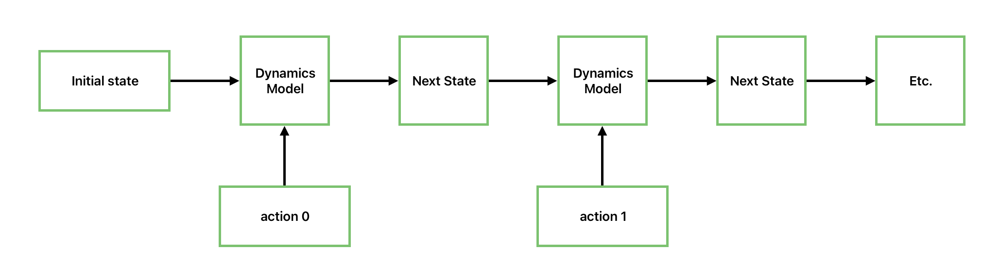
Let’s start with the basics first. The goal of MBRL is to learn a model of the environment. The idea being that if you had a perfect model of the environment, then you could use that to plan a sequence of actions to get to your desired goal state. The difficulty is now to train that model, which should take in the current state and the performed action as input and predict the next state . For this, we will just use a simple MLP (btw. we are training on CartPole for now - gotta start somewhere, right?):
class DynamicsModel(eqx.Module):
    mlp: eqx.nn.MLP

    n_dims: int = eqx.field(static=True)
    n_actions: int = eqx.field(static=True)

    def __init__(self, n_dims: int, n_actions: int, key: PRNGKeyArray):
        self.mlp = eqx.nn.MLP(
            in_size=n_dims + n_actions,
            out_size=n_dims,
            width_size=32,
            depth=2,
            key=key,
        )
        self.n_dims = n_dims
        self.n_actions = n_actions

    def __call__(self, x: Float[Array, " n_dims+n_actions"]) -> Float[Array, "n_dims"]:
        state = x[: self.n_dims]
        delta = self.mlp(x)
        return state + delta
Admittedly, this is not the purest MLP, because we are using residual connections, i.e. we are trying to learn the delta between the current state and the next state. The argument is that usually there is not such a drastic change between states, thus being easier to learn the delta than the whole thing.
Ok, so now we have a dynamics prediction model (we have no idea yet if it works or not though). One thing we will need for sure is data! One of the advantages of MBRL is that all data is good data, in the sense that you have no reason to throw out any data, since all the data you collect comes from the environment i.e. the ground truth.
def collect_data(
    env: gym.Env,
    n_episodes: int,
    dynamics_model,
    reward_model,
    epsilon: float = 0.1,
    n_horizon: int = 10,
) -> list[tuple[Array, Array, Array, Array]]:
    data = []
    for i in range(n_episodes):
        state, _ = env.reset()

        terminated, truncated = False, False
        while not terminated and not truncated:
            if random.random() < epsilon:
                action = env.action_space.sample()
            else:
                action = int(????)
            next_state, reward, terminated, truncated, _ = env.step(action)
            data.append((state, action, reward, next_state))
    return data
The above function is simple: just create n_episode worth of data using epsilon-greedy exploration, i.e. 10 % random exploration (in this example). But what about the else part?
In the else branch, we have to specify how we should - in general - choose actions based on our model. I alluded to this earlier, namely that we need to plan ahead. Following the talk from Sergey Levine, you could use the cross-entropy method (CEM), which is a gradient-free planning method, although there are certainly other methods as well, such as Monte-Carlo Tree Search (MCTS). We will use CEM for now and later use MCTS to see the difference.
Excursion: Cross-Entropy Method
CEM is a planning algorithm with the goal to give us the best action to take at the current state. It’s an iterative process, starting with a uniform distribution of actions and then morphing that into the best possible action probabilities (hence the name cross-entropy - you are trying to minimise the difference between a uniform distrubtion and the best distribution).
We need to give the algorithm also n_horizon which refers to how many steps into the future you should plan ahead. One of the problems with MBRL is compounding errors - namely the future ahead you plan, the more the small errors from your dynamics model pile up, eventually given a prediction which could be far away from the truth (software developers have the same problem - rarely have plans for a projects worked and yet we throw shade at MBRL algorithms for not being able to plan ahead…).
@eqx.filter_jit
def reward_model_planning(
    dynamics_model: DynamicsModel,
    reward_model: RewardModel,
    initial_state: Array,
    n_horizon: int = 10,
    n_samples: int = 100,
    n_iterations: int = 5,
    n_elite: int = 10,
    n_actions: int = 2,
):
Wait, what the hell is this RewardModel - you might be asking, rightfully so since I haven’t introduced that yet.
We are trying to plan ahead into the future and evaluate each trajectory. But how good is the trajectory?
Our dynamics model can predict the next state, but it can’t predict the next reward. What makes this situation even more difficult is that in our environment (i.e. CartPole) the reward is always . So, our reward model looks like this:
class RewardModel(eqx.Module):
    mlp: eqx.nn.MLP

    n_dims: int = eqx.field(static=True)
    n_actions: int = eqx.field(static=True)

    def __init__(self, n_dims: int, n_actions: int, key: PRNGKeyArray):
        self.mlp = eqx.nn.MLP(
            in_size=n_dims + n_actions,
            out_size=1,
            width_size=32,
            depth=2,
            key=key,
        )
        self.n_dims = n_dims
        self.n_actions = n_actions

    def __call__(self, x: Float[Array, "n_dims+n_actions"]) -> Float[Array, ""]:
        return self.mlp(x)
And it takes as input the current state and action and returns a scalar, which is the predicted reward. Later, during training, you will notice that the loss of this reward model quickly drops to 0 so it’s actually not all that useful (it’s not that hard to predict 1 every single time). A much better way to estimate reward for the CartPole environment would be to make it dependent on the angle and velocity of the cart. But hand crafting rewards like this will quickly fall apart and does not scale and is not general enough (what’s the ideal reward function for LunarLander?).
But because we have no other option right now, we will use this reward model.
Now comes the initial action probability.
action_probs = jnp.ones((n_horizon, n_actions)) / n_actions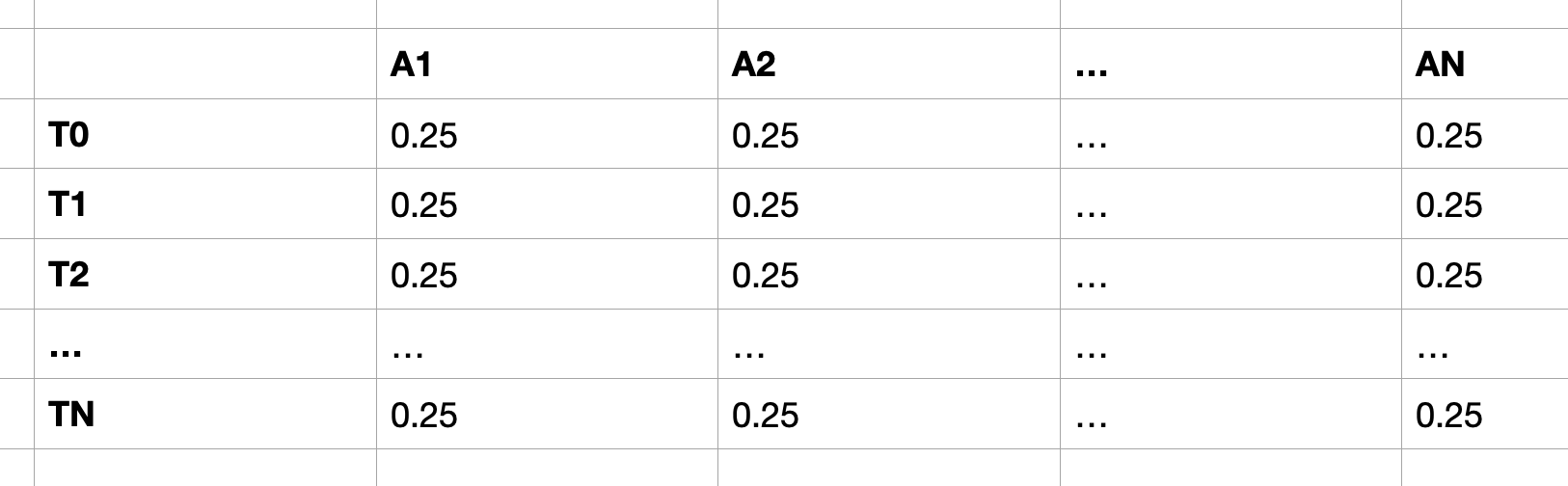
These numbers assume n_actions=4 and the y axis corresponds to the timesteps while the x axis is the probability for that action at that timestep. The goal is to find the “optimal” action probabilities, e.g.:
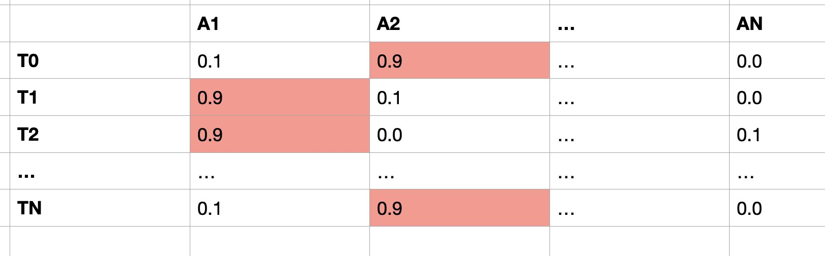
In this example, the best action sequence to pick is at , at , at and so on and lastly at
In my implementation, since I use JAX, there are a few JAX-ish things happening, lots of vmap and jax.lax.scan action going on. We can leverage these to parallelise a lot of computations and we can do that, because the CEM algorithm doesn’t depend on the actual environment - that’s what we use the dynamics model for.
Ok so here’s the entire code and I will cover a few of the more relevant parts of it:
def reward_model_planning(
    dynamics_model: DynamicsModel,
    reward_model: RewardModel,
    initial_state: Array,
    n_horizon: int = 10,
    n_samples: int = 100,
    n_iterations: int = 5,
    n_elite: int = 10,
    n_actions: int = 2,
):
    action_probs = jnp.ones((n_horizon, n_actions)) / n_actions

    def simulate_step(action_sequences: Array, dynamics_model, reward_model):
        def step_trajectory(state_and_idx, timestep):
            sample_idx, current_state = state_and_idx
            action = action_sequences[sample_idx, timestep]

            action_one_hot = jnp.zeros(n_actions)
            action_one_hot = action_one_hot.at[action].set(1.0)
            model_input = jnp.concatenate([current_state, action_one_hot])

            reward = reward_model(model_input)
            next_state = dynamics_model(model_input)

            return (sample_idx, next_state), reward

        return step_trajectory

    def evaluate_trajectory(sample_idx, trajectory_stepper):
        state = initial_state
        _, rewards = jax.lax.scan(
            f=trajectory_stepper, init=(sample_idx, state), xs=jnp.arange(n_horizon)
        )
        total_reward = jnp.sum(rewards)
        return total_reward

    def iterate(carry, x):
        action_probs = carry
        keys = jax.random.split(jax.random.PRNGKey(x), n_samples)

        def sample_actions(key):
            return jax.vmap(
                lambda p, k: jax.random.choice(k, jnp.arange(n_actions), p=p)
            )(action_probs, jax.random.split(key, n_horizon))

        action_sequences = jax.vmap(sample_actions)(keys)
        trajectory_stepper = simulate_step(
            action_sequences, dynamics_model, reward_model
        )
        trajectory_evaluator = functools.partial(
            evaluate_trajectory, trajectory_stepper=trajectory_stepper
        )
        trajectory_rewards = eqx.filter_vmap(trajectory_evaluator)(
            jnp.arange(n_samples)
        )

        elite_indices = jnp.argsort(trajectory_rewards)[-n_elite:]
        elite_actions = action_sequences[elite_indices]
        action_probs = jnp.mean(elite_actions, axis=0)
        new_action_probs = jnp.zeros_like(action_probs)
        elite_actions_one_hot = jax.nn.one_hot(elite_actions, n_actions)
        new_action_probs = jnp.mean(elite_actions_one_hot, axis=0)

        return new_action_probs, None

    action_probs, _ = jax.lax.scan(
        iterate, init=(action_probs), xs=jnp.arange(n_iterations)
    )

    keys = jax.random.split(jax.random.PRNGKey(n_iterations), n_samples)

    def sample_final_actions(key):
        return jax.vmap(lambda p, k: jax.random.choice(k, jnp.arange(n_actions), p=p))(
            action_probs, jax.random.split(key, n_horizon)
        )

    final_action_sequences = jax.vmap(sample_final_actions)(keys)

    final_trajectory_stepper = simulate_step(
        final_action_sequences, dynamics_model, reward_model
    )
    final_evaluator = functools.partial(
        evaluate_trajectory, trajectory_stepper=final_trajectory_stepper
    )
    final_rewards = eqx.filter_vmap(final_evaluator)(jnp.arange(n_samples))
    best_idx = jnp.argmax(final_rewards)
    best_first_action = final_action_sequences[best_idx, 0]
    return best_first_action
The top level call to get the action_probs is this
action_probs, _ = jax.lax.scan(
        iterate, init=(action_probs), xs=jnp.arange(n_iterations)
    )
If you didn’t know, jax.lax.scan is a JAX primitive and I have created a video on that - it kind of works like a for loop with a carry. The function we use in the loop is the iterate function.
In the iterate function, we first sample the actions to get the action_sequences array which has the shape n_samples x n_horizon.
This part
trajectory_stepper = simulate_step(
    action_sequences, dynamics_model, reward_model
)
creates the stepper function, which will be called inside the evaluate_trajectory function:
def evaluate_trajectory(sample_idx, trajectory_stepper):
    state = initial_state
    _, rewards = jax.lax.scan(
        f=trajectory_stepper, init=(sample_idx, state), xs=jnp.arange(n_horizon)
    ) # basically just simulate n_horizon steps
    total_reward = jnp.sum(rewards)
    return total_reward
Inside the trajectory_stepper function, we use the dynamics model to estimate the next state and use the reward model to estimate the reward, which in turn tells us how good this specific trajectory is.
With this vmap
trajectory_rewards = eqx.filter_vmap(trajectory_evaluator)(
    jnp.arange(n_samples)
)
We compute all the trajectories (i.e. all the samples) in parallel and we can do that because each sample is independent of each other. Very efficient stuff!
This part
elite_indices = jnp.argsort(trajectory_rewards)[-n_elite:]
elite_actions = action_sequences[elite_indices]
action_probs = jnp.mean(elite_actions, axis=0)
new_action_probs = jnp.zeros_like(action_probs)
elite_actions_one_hot = jax.nn.one_hot(elite_actions, n_actions)
new_action_probs = jnp.mean(elite_actions_one_hot, axis=0)

return new_action_probs, None
basically just gets the best trajectories and computes the average of the best action probabilities (this is the cross-entropy part).
We then do one last evaluation, to get the best action:
action_probs, _ = jax.lax.scan(
    iterate, init=(action_probs), xs=jnp.arange(n_iterations)
)

keys = jax.random.split(jax.random.PRNGKey(n_iterations), n_samples)

def sample_final_actions(key):
    return jax.vmap(lambda p, k: jax.random.choice(k, jnp.arange(n_actions), p=p))(
        action_probs, jax.random.split(key, n_horizon)
    )

final_action_sequences = jax.vmap(sample_final_actions)(keys)

final_trajectory_stepper = simulate_step(
    final_action_sequences, dynamics_model, reward_model
)
final_evaluator = functools.partial(
    evaluate_trajectory, trajectory_stepper=final_trajectory_stepper
)
final_rewards = eqx.filter_vmap(final_evaluator)(jnp.arange(n_samples))
best_idx = jnp.argmax(final_rewards)
best_first_action = final_action_sequences[best_idx, 0]
return best_first_action
Back to MBRL
There are a few things we could improve in the CEM algorithm but the biggest issue is the way we compute the rewards, which is kind of meaningless: it does not differentiate between the pole being upright in the middle and being almost horizontal; in both cases you get a reward of 1. Ideally, you should get more reward the slower and vertical the pole is.
Let’s update the collect_data function:
def collect_data(
    env: gym.Env,
    n_episodes: int,
    dynamics_model,
    reward_model,
    epsilon: float = 0.1,
    n_horizon: int = 10,
) -> list[tuple[Array, Array, Array, Array]]:
    data = []
    for i in range(n_episodes):
        state, _ = env.reset()

        terminated, truncated = False, False
        while not terminated and not truncated:
            if random.random() < epsilon:
                action = env.action_space.sample()
            else:
                action = int(
                    reward_model_planning(
                        dynamics_model, reward_model, state, n_horizon=n_horizon
                    )
                )
            next_state, reward, terminated, truncated, _ = env.step(action)
            data.append((state, action, reward, next_state))
    return data
Assuming we have some data, we then need to train the models. This is standard JAX boilerplate. We use MSE loss for both models:
@eqx.filter_value_and_grad
def mse_loss(model, x, y):
    preds = jax.vmap(model)(x)
    return jnp.mean((preds - y) ** 2)


@eqx.filter_jit
def step(model, x, y, opt_state, optimizer):
    loss, grads = mse_loss(model, x, y)
    updates, opt_state = optimizer.update(grads, opt_state)
    model = eqx.apply_updates(model, updates)
    return model, opt_state, loss


def train_models(
    data,
    dynamics_model,
    reward_model,
    n_epochs,
    batch_size,
    learning_rate,
    optimizer,
    dynamics_opt_state,
    reward_opt_state,
):
    states = jnp.array([d[0] for d in data])
    actions = jnp.array([d[1] for d in data])
    rewards = jnp.array([d[2] for d in data])
    next_states = jnp.array([d[3] for d in data])

    actions_onehot = jax.vmap(lambda a: jax.nn.one_hot(a, dynamics_model.n_actions))(
        actions
    )
    inputs = jnp.concatenate([states, actions_onehot], axis=1)

    metrics = LossMetrics.empty()

    for epoch in range(n_epochs):
        idx = jax.random.permutation(jax.random.PRNGKey(epoch), jnp.arange(len(data)))
        batches = 0

        for i in range(0, len(data), batch_size):
            batch_idx = idx[i : i + batch_size]
            batches += 1

            batch_inputs = inputs[batch_idx]
            batch_targets = next_states[batch_idx]
            dynamics_model, dynamics_opt_state, d_loss = step(
                dynamics_model,
                batch_inputs,
                batch_targets,
                dynamics_opt_state,
                optimizer,
            )

            batch_rewards = rewards[batch_idx]
            reward_model, reward_opt_state, r_loss = step(
                reward_model, batch_inputs, batch_rewards, reward_opt_state, optimizer
            )

            metrics = metrics.merge(
                LossMetrics.single_from_model_output(
                    dynamic_loss=d_loss, reward_loss=r_loss
                )
            )

    return dynamics_model, reward_model, metrics, dynamics_opt_state, reward_opt_state
Finally, we train the whole thing:
def model_based_rl(
env,
n_iterations: int,
n_initial_episodes: int,
n_model_steps: int,
n_additional_episodes: int,
epsilon: float,
n_epochs: int,
batch_size: int,
learning_rate: float,
n_horizon: int,
):
state_dim = env.observation_space.shape[0]
action_dim = env.action_space.n
dynamics_model = DynamicsModel(
n_dims=int(state_dim), n_actions=int(action_dim), key=jax.random.key(0)
)
reward_model = RewardModel(
n_dims=int(state_dim), n_actions=int(action_dim), key=jax.random.key(1)
)
optimizer = optax.adam(learning_rate)
dynamics_opt_state = optimizer.init(eqx.filter(dynamics_model, eqx.is_array))
reward_opt_state = optimizer.init(eqx.filter(reward_model, eqx.is_array))
data = collect_data(
env,
n_initial_episodes,
dynamics_model,
reward_model,
epsilon,
n_horizon=n_horizon,
)
reward_metrics = RewardMetrics.empty()
for iteration in range(n_iterations):
dynamics_model, reward_model, metrics, dynamics_opt_state, reward_opt_state = (
train_models(
data,
dynamics_model,
reward_model,
n_epochs,
batch_size,
learning_rate,
optimizer,
dynamics_opt_state,
reward_opt_state,
)
)
losses_computed = metrics.compute()
new_data = collect_data(
env,
n_additional_episodes,
dynamics_model,
reward_model,
epsilon,
n_horizon=n_horizon,
)
data.extend(new_data)
eval_rewards = evaluate_policy(env, dynamics_model, reward_model)
reward_metrics = reward_metrics.merge(
RewardMetrics.single_from_model_output(rewards=eval_rewards)
)
rewards_computed = reward_metrics.compute()
print(losses_computed, rewards_computed)
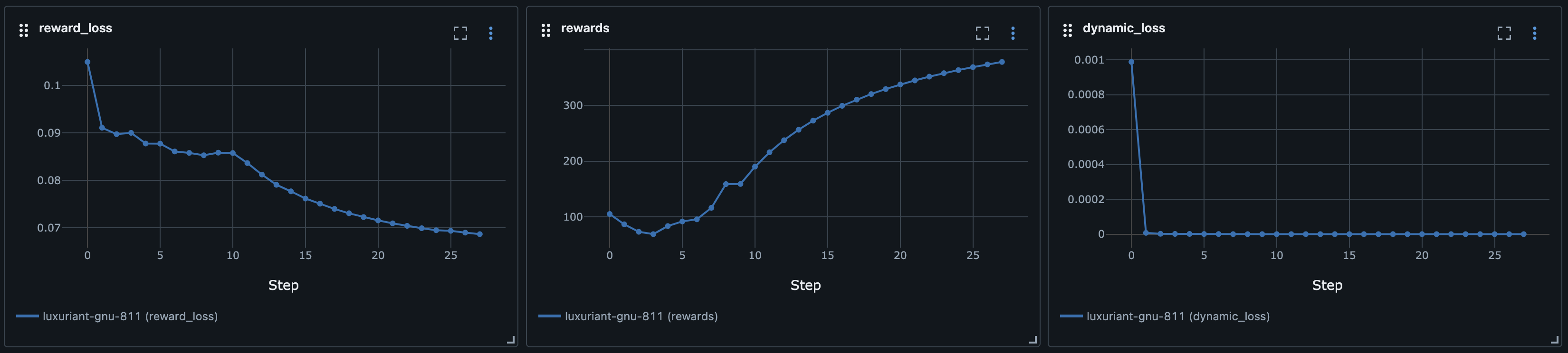
return dynamics_model, reward_modelIf you train the whole thing, you will get graphs like these:
Dynamics loss

Rewards loss

Rewards

Pretty bad, right? Well, yes. Let’s try to change the reward function a bit to make it dependent on the position of the cart and pole to see if that improves things.
Rewards (using a slightly larger dynamics model)

Something definitely changed, namely the reward never dipped below 50, whereas in the previous approach with the reward model, the performance just kept getting worse. But it’s not feasible to hand craft the reward model every time. In this example it was just a simple matter of asking Claude if it can just code it out for me, but that won’t always be possible.
Little GIF
What does the dynamics model actually predict? I collected some data for state transitions from the actual environment and what the dynamics model predicts. Have a look at these examples:
I have to say I like these predictions. Sure, they are “over the top” and predict a super drastic change in the cart, but it looks like the physics kind of checks out, especially in the second GIF. Look at how if the pole is tilted to the right and if the cart moves to the right, then the pole moves to the left!
Conclusion (for now)
This was expected. Sergey said as much in his talk in the linked video that MBRL - in this basic setting - does not work and I have to concur. But the MBRL journey is far from done. For one, we can switch CEM with MCTS to get potentially better results (for reference, AlphaGo used MCTS) but we can also use the other tricks that Sergey and their team have found. We will see about that in the next post.
Errata
Ouch. I just saw that I had a major flaw in my data collection pipeline, which is the entire reason, that the dynamics model got “stuck” and didn’t improve any further beyond a loss of around 0.2.
Looking at this code again
def collect_data(
    env: gym.Env,
    n_episodes: int,
    dynamics_model,
    reward_model,
    epsilon: float = 0.1,
    n_horizon: int = 10,
) -> list[tuple[Array, Array, Array, Array]]:
    data = []
    for i in range(n_episodes):
        state, _ = env.reset()

        terminated, truncated = False, False
        while not terminated and not truncated:
            if random.random() < epsilon:
                action = env.action_space.sample()
            else:
                action = int(
                    reward_model_planning(
                        dynamics_model, reward_model, state, n_horizon=n_horizon
                    )
                )
            next_state, reward, terminated, truncated, _ = env.step(action)
            data.append((state, action, reward, next_state))
    return data
We can see that we predict the action like this
reward_model_planning(
    dynamics_model, reward_model, state, n_horizon=n_horizon
)
But the issue is that state is always the initial state! It never gets updated. Furthermore, this line
data.append((state, action, reward, next_state))makes everything worse, because state is the initial state of the environment and next_state keeps changing, so it’s a miracle at all that I got some high returns at all. A simple fix for this is:
state = next_stateWith that single line added, the MBRL algorithm works and really soars:
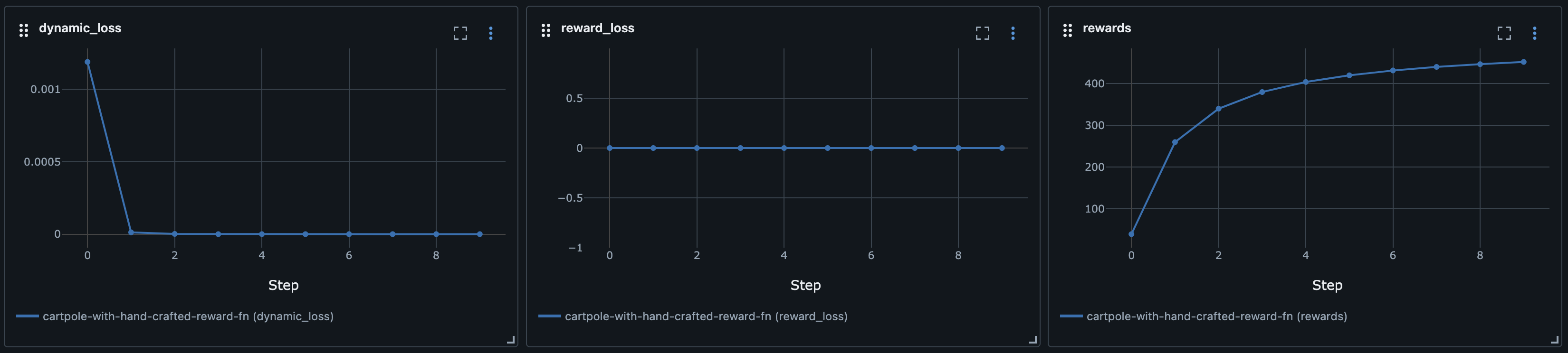
This is using the hand-crafted reward signal. If we run the same code again with the reward model, we can see just how badly it performs:
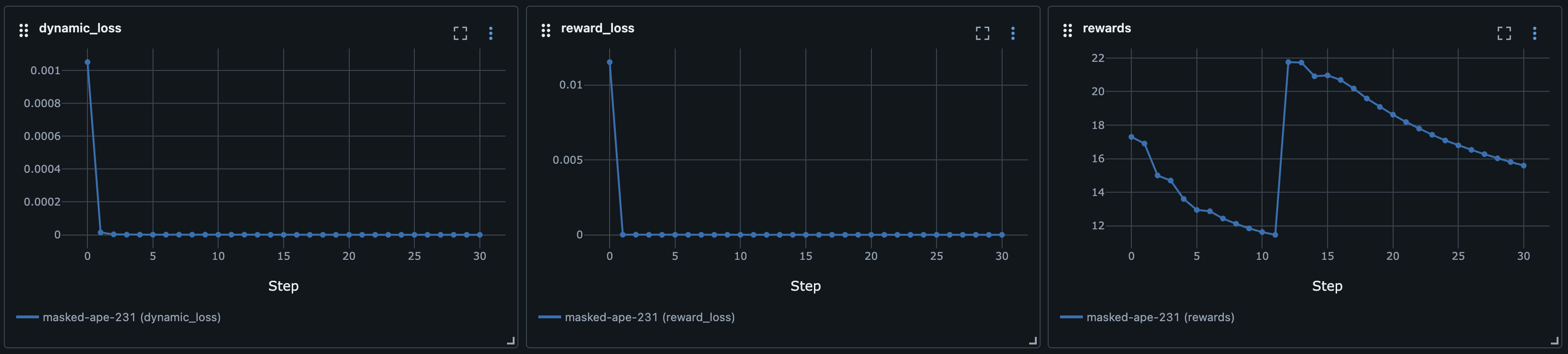
This just goes to show how important a good reward signal is during planning. In both cases, the dynamics model learned the model just fine (very low loss), but the planning is what leads to the low returns, because the reward signal is not helpful at all and is not properly guiding the planning step.
But you can actually remedy this by changing the way you collect the data. For instance if you used this data collection:
def collect_data(
    env: gym.Env,
    n_episodes: int,
    dynamics_model,
    reward_model,
    epsilon: float = 0.1,
    n_horizon: int = 10,
    gamma: float = 0.99,
) -> list[tuple[Array, Array, Array, Array, Array]]:
    data = []
    for i in range(n_episodes):
        state, _ = env.reset()
        episode_data = []

        terminated, truncated = False, False
        while not terminated and not truncated:
            if random.random() < epsilon:
                action = env.action_space.sample()
            else:
                action = int(
                    reward_model_planning(
                        dynamics_model, reward_model, state, n_horizon=n_horizon
                    )
                )
            next_state, reward, terminated, truncated, _ = env.step(action)
            episode_data.append((state, action, reward, next_state))
            state = next_state

        # Calculate returns
        returns = []
        G = 0
        for s, a, r, ns in reversed(episode_data):
            G = r + gamma * G
            returns.insert(0, G)

        if returns:
            max_return = max(returns)
            min_return = min(returns)
            # Avoid division by zero
            if max_return > min_return:
                normalized_returns = [
                    (r - min_return) / (max_return - min_return) for r in returns
                ]
            else:
                normalized_returns = [1.0 for _ in returns]
        else:
            normalized_returns = []

        for (s, a, r, ns), g in zip(episode_data, normalized_returns):
            data.append((s, a, r, ns, g))

    return data
Then you would calculate the expected future rewards given a state . This way, you introduce the idea that if the pole is upright in the middle, then this will likely yield higher results in the future. Then, of course, you have to change the training part a bit:
def train_models(
    data,
    dynamics_model,
    reward_model,
    n_epochs,
    batch_size,
    learning_rate,
    optimizer,
    dynamics_opt_state,
    reward_opt_state,
):
    states = jnp.array([d[0] for d in data])
    actions = jnp.array([d[1] for d in data])
    rewards = jnp.array([d[2] for d in data])
    next_states = jnp.array([d[3] for d in data])
    returns = jnp.array([d[4] for d in data])

    actions_onehot = jax.vmap(lambda a: jax.nn.one_hot(a, dynamics_model.n_actions))(
        actions
    )
    inputs = jnp.concatenate([states, actions_onehot], axis=1)

    metrics = LossMetrics.empty()

    for epoch in range(n_epochs):
        idx = jax.random.permutation(jax.random.PRNGKey(epoch), jnp.arange(len(data)))
        batches = 0

        for i in range(0, len(data), batch_size):
            batch_idx = idx[i : i + batch_size]
            batches += 1

            batch_inputs = inputs[batch_idx]
            batch_targets = next_states[batch_idx]
            dynamics_model, dynamics_opt_state, d_loss = step(
                dynamics_model,
                batch_inputs,
                batch_targets,
                dynamics_opt_state,
                optimizer,
            )

            batch_returns = returns[batch_idx]
            reward_model, reward_opt_state, r_loss = step(
                reward_model, batch_inputs, batch_returns, reward_opt_state, optimizer
            ) # train on the returns now!

            metrics = metrics.merge(
                LossMetrics.single_from_model_output(
                    dynamic_loss=d_loss, reward_loss=r_loss
                )
            )

    return dynamics_model, reward_model, metrics, dynamics_opt_state, reward_opt_state
When you do this instead, the model solves the environment as well: