Monte-Carlo Tree Search (DRAFT)

Monte-Carlo Tree Search (MCTS) is an incredible planning algorithm that was successfully used in AlphaGo a couple of years (almost a decade ago), which was responsible for beating expert humans in the game of Go.

In this post, we will cover and implement a simple and modular library for MCTS.

What is a Tree in MCTS?

A tree in MCTS consists of nodes and edges, like any other tree except those found in nature. Each node corresponds uniquely to a state in your environment, like a chess game state or your current position in FrozenLake. The edges are the actions that you can perform.

In our code, we need some arrays that hold information about the tree structure (which we will use to traverse the tree) and also some metrics about the nodes and edges (such as how often was a node visited).

In Python, our tree is defined as this:

@dataclass
class Tree:
    # Tree structure arrays
    parent_indices: list[int] # n x 1
    children_indices: list[list[int]] # n x a
    action_from_parent: list[int] # n x 1

    # Tree data
    n_s: list[int] # n x 1
    n_sa: list[list[int]] # n x a

    v_s: list[float] # n x 1
    q_sa: list[list[float]] # n x a
    r_sa: list[list[float]] # n x a

    dones: list[bool] # n x 1
    states: dict[int, Any]

Parent Indices

The parent indices array tells us what the INDEX of the parent is of any node in our tree.

Here’s an example:

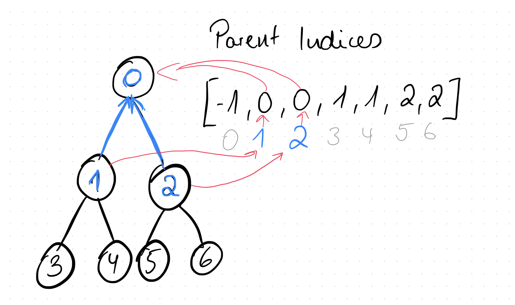
The content of the parent_indices array contains the indices of the parents of the nodes. E.g. the node with index 2 has parent 0. This means we check the array at index 2 and see that the value of that is 0. If we now checked the parent_indices array at position 0 to get the “grand parent”, we see it says -1, which is the case because the root node has no parent (hence the “special” value of -1).

Children Indices

As the name suggests, this is a $n \times a$ array, where $n$ is the number of nodes in the tree and $a$ is the number of available actions. This array gives us the indices of all the children of any node.

Here’s an example:

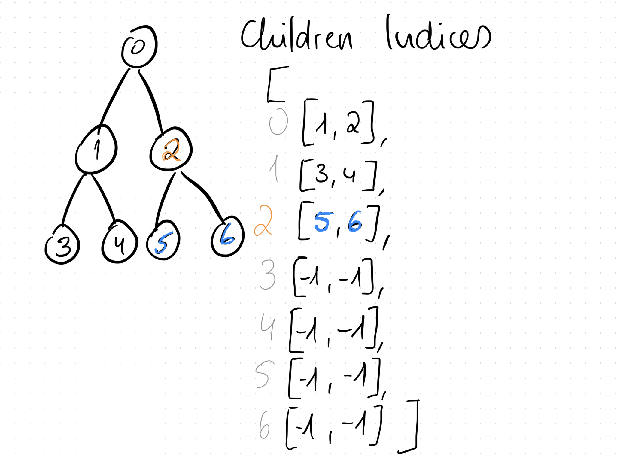
In this example, if we check the index 2, we see that it contains an array with the values [5, 6], which means that the children of node 2 are 5 and 6. If a node has no children, they get the special value of -1.

Action from Parent

This is the last array that we need to traverse our tree. This one tells us what action to perform from the perspective of the parent to reach the current node. Here’s another example:

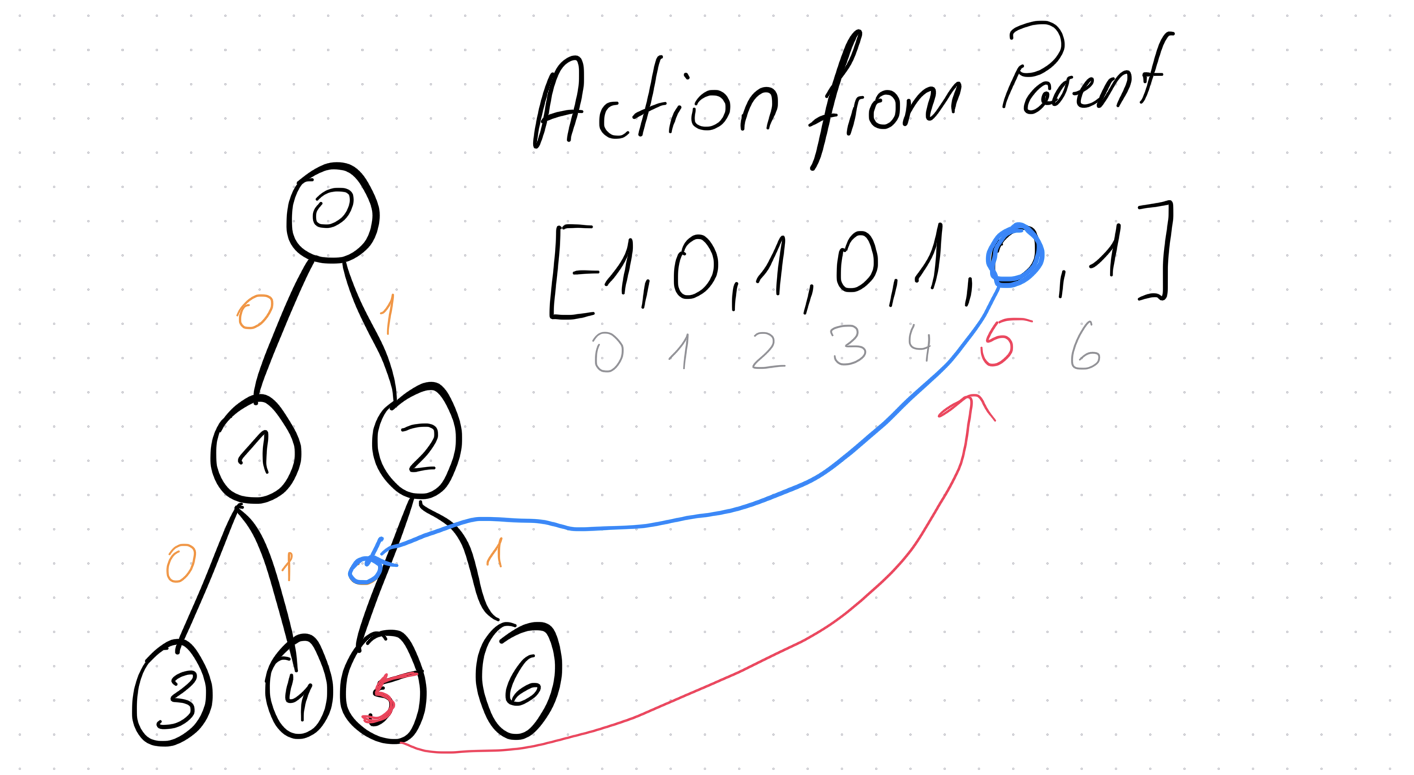
In this example, to get to node 5, the parent needs to perform action 0, thus action_from_parent[5] = 0.

Tree Data

Let’s quickly walk through the metrics that we need to collect in our tree.

n_s: list[int] # n x 1
n_sa: list[list[int]] # n x a

These are visit counters. $N(s)$ gives us the number of times that node $s$ was visited. $N(s,a)$ gives us the number of times the state-action pair $s,a$ was visited.

v_s: list[float] # n x 1
q_sa: list[list[float]] # n x a
r_sa: list[list[float]] # n x a

For these, I chose to go with the RL notation. $V(s)$ is the value of a node, similar to what it means in reinforcement learning; you could also name this node_values. $Q(s,a)$ is the value of picking action $a$ while in state $s$; another name for this could be children_values. Lastly, $R(s,a)$ gives us the reward for picking action $a$ in state $s$.

dones: list[bool] # n x 1
states: dict[int, Any]

The dones array contains flags if a state $s$ is terminal (so that we can stop MCTS early). Finally, states is a mapping from a node index to whatever representation of your state the environment has. E.g. for chess that chould be a 2x2 matrix containing information of the board, whereas for FrozenLake is the current position of your character. We use Any because we don’t know - or care - what this data will be; we don’t care about it, because in the end, only the user’s code will be interacting with this data and not our MCTS algorithm.

Let’s initialise our tree:

def generate_tree(n_nodes: int, n_actions: int, root_fn_output: RootFnOutput) -> Tree:
    parent_indices = [NO_PARENT for _ in range(n_nodes)]
    action_from_parent = [NO_PARENT for _ in range(n_nodes)]
    children_indices = [[UNVISITED for __ in range(n_actions)] for _ in range(n_nodes)]

    n_s = [0 for _ in range(n_nodes)]
    v_s = [0.0 for _ in range(n_nodes)]

    q_sa = [[0.0 for __ in range(n_actions)] for _ in range(n_nodes)]
    n_sa = [[0 for __ in range(n_actions)] for _ in range(n_nodes)]
    r_sa = [[0.0 for __ in range(n_actions)] for _ in range(n_nodes)]
    dones = [False for _ in range(n_nodes)]

    states = {ROOT_INDEX: root_fn_output.state}

    return Tree(
        parent_indices=parent_indices,
        children_indices=children_indices,
        action_from_parent=action_from_parent,
        n_s=n_s,
        v_s=v_s,
        dones=dones,
        q_sa=q_sa,
        n_sa=n_sa,
        r_sa=r_sa,
        states=states,
    )

Now that we have looked at our tree, it’s time to go over the steps in MCTS.

The MCTS Algorithm

MCTS consists of 4 steps in this order:

1. Selection
2. Expansion
3. Simulation
4. Backpropagation

On a high level, the algorithm - written in this search method, looks like this

class MCTS:
    @staticmethod
    def search(
        n_actions: int,
        root_fn: Callable[[], RootFnOutput],
        policy_fn: Callable[[PolicyInput], PolicyReturn],
        step_fn: Callable[[StepFnInput], StepFnReturn],
        max_depth: int,
        n_iterations: int,
    ):
        node_index_counter = 0
        tree = generate_tree(
            n_nodes=n_iterations + 1, n_actions=n_actions, root_fn_output=root_fn()
        )

        for iteration in range(n_iterations):
            selection_output = selection(tree, max_depth, policy_fn)

            if (
                tree.children_indices[selection_output.parent_index][
                    selection_output.action
                ]
                == UNVISITED
            ):
                node_index_counter += 1
                leaf_node = expansion(
                    tree, selection_output, node_index_counter, step_fn
                )
            else:
                child_idx = tree.children_indices[selection_output.parent_index][
                    selection_output.action
                ]
                leaf_node = LeafNode(
                    node_index=child_idx,
                    action=selection_output.action,
                )

            tree = backpropagate(tree, leaf_node.node_index)

        return tree

Let’s go over this function briefly, before deep-diving into the individual steps:

In this section, we first initialise the tree. The maximum number of nodes the tree will have is the number of expansions we perform, which is at most the number of iterations.

class MCTS:
    @staticmethod
    def search(
        n_actions: int,
        root_fn: Callable[[], RootFnOutput],
        policy_fn: Callable[[PolicyInput], PolicyReturn],
        step_fn: Callable[[StepFnInput], StepFnReturn],
        max_depth: int,
        n_iterations: int,
    ):
        node_index_counter = 0
        tree = generate_tree(
            n_nodes=n_iterations + 1, n_actions=n_actions, root_fn_output=root_fn()
        )

These are the functions that we expect from the user:

RootFnOutput = NamedTuple("RootFnOutput", [("state", Any)])

root_fn: Callable[[], RootFnOutput], # required to initialise the tree
policy_fn: Callable[[PolicyInput], PolicyReturn], # required in selection - see later
step_fn: Callable[[StepFnInput], StepFnReturn], # required in expansion - see later

The following is the main loop of MCTS:

for iteration in range(n_iterations):
    selection_output = selection(tree, max_depth, policy_fn)

    if (
        tree.children_indices[selection_output.parent_index][
            selection_output.action
        ]
        == UNVISITED
    ):
        node_index_counter += 1
        leaf_node = expansion(
            tree, selection_output, node_index_counter, step_fn
        )
    else:
        child_idx = tree.children_indices[selection_output.parent_index][
            selection_output.action
        ]
        leaf_node = LeafNode(
            node_index=child_idx,
            action=selection_output.action,
        )

    tree = backpropagate(tree, leaf_node.node_index)

Let’s go over each of these steps.

Selection

The goal of the selection step is to find an unvisited node - or stop if we can’t find one (e.g. because we have already explored the entire tree or we have reached some max_depth).

This step is used in this section of the main MCTS loop:

for iteration in range(n_iterations):
    selection_output = selection(tree, max_depth, policy_fn)

Initially, all the nodes in the tree are unvisited, including the root node. But let’s say we already did a couple of iterations of MCTS and have explored and added a bunch of nodes to our tree, then the question is: how do we traverse the tree?

Say you are at the root node:

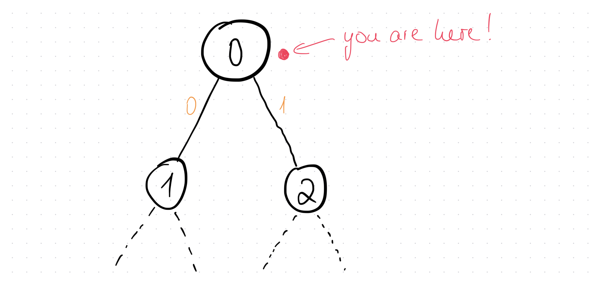
How do you chose, which path to go down? What’s the strategy? You have a bunch of stored metrics about the tree that you can make use of. One strategy might even be something like “if the state visit count of my current node (root in this example) is even, go left (pick action 0), else go right (action 1)”. Or you could also just pick the action that was visited less (i.e. check the n_sa array like min(n_sa[0])).

But how do we decide? The answer is that we don’t! We let the user decide and simply tell us the action that we need to take!

To clarify what I mean by this, let’s have a look at the function signature of the selection function:

PolicyInput = NamedTuple(
    "PolicyInput", [("tree", Tree), ("node_index", int), ("depth", int)]
)
PolicyReturn = NamedTuple("PolicyReturn", [("action", int)])
SelectionOutput = NamedTuple(
    "SelectionOutput", [("parent_index", int), ("action", int)]
)

def selection(
    tree: Tree,
    max_depth: int,
    policy_fn: Callable[[PolicyInput], PolicyReturn],
) -> SelectionOutput:
    ...

The policy_fn is an argument that we expect from our user. Basically, we will give the user the tree, the current node as well as the current depth and in return, the user will give us the action to perform. A popular policy_fn is e.g. the UCB1 function. We can provide a sample implementation that the user can choose to use, or the user will simply give us their own version. Regardless, in the end, we have a function that we can call, which will give us the action.

From here, the rest of the function is extremely simple:

def selection(
    tree: Tree,
    max_depth: int,
    policy_fn: Callable[[PolicyInput], PolicyReturn],
) -> SelectionOutput:
    n = ROOT_INDEX # we start at the root node
    p = NO_PARENT # = -1
    a = UNVISITED # = -1
    depth = 0

    while True:
        # if we reach max depth or terminal state, end early
        if tree.dones[n] or depth >= max_depth:
            return SelectionOutput(p, a)

        # get the action
        policy = policy_fn(PolicyInput(tree, n, depth))

        # get the child
        c = tree.children_indices[n][policy.action]

        if c == UNVISITED:
            # if child was not visited before
            # return the node and the action
            return SelectionOutput(n, policy.action)
        else:
            p = n # next iteration's parent is the current node
            n = c # next iteration's current node is the child
            a = policy.action
            depth += 1 # increment the depth

Basically, just keep picking the child and go deeper down the tree, until we reach the maximum depth or a terminal node OR an unvisited node.

Expansion (and Simulation)

Once we have selected a node and have our SelectionOutput it’s time to expand the node - if possible.

This step is used in this section of the main MCTS loop:

if (
    tree.children_indices[selection_output.parent_index][
        selection_output.action
    ]
    == UNVISITED
):
    node_index_counter += 1

    # EXPAND ONLY IF UNVISITED NODE AND CREATE NEW LEAF NODE

    leaf_node = expansion(
        tree, selection_output, node_index_counter, step_fn
    )
else:
    # OTHERWISE DON'T EXPAND; USE LEAF DIRECTLY
    child_idx = tree.children_indices[selection_output.parent_index][
        selection_output.action
    ]
    leaf_node = LeafNode(
        node_index=child_idx,
        action=selection_output.action,
    )

The expansion function is fairly straightforward:

StepFnInput = NamedTuple("StepFnInput", [("state", Any), ("action", int)])
StepFnReturn = NamedTuple(
    "StepFnReturn",
    [("value", float), ("reward", float), ("done", bool), ("state", Any)],
)


def expansion(
    tree: Tree,
    selection_output: SelectionOutput,
    next_node_index: int,
    step_fn: Callable[[StepFnInput], StepFnReturn],
) -> LeafNode:
    parent_index, action = selection_output
    assert tree.children_indices[parent_index][action] == UNVISITED, (
        f"Can only expand unvisited nodes, got {tree.children_indices[parent_index][action]=}"
    )
    state = tree.states[parent_index]
    value, reward, done, next_state = step_fn(StepFnInput(state=state, action=action))
    tree.children_indices[parent_index][action] = next_node_index
    tree.action_from_parent[next_node_index] = action
    tree.parent_indices[next_node_index] = parent_index
    tree.v_s[next_node_index] = value
    tree.n_s[next_node_index] = 1
    tree.dones[next_node_index] = done
    tree.r_sa[parent_index][action] = reward
    tree.states[next_node_index] = next_state

    return LeafNode(
        node_index=next_node_index,
        action=action,
    )

Essentially, we ask from the user to give as a step_fn. What we need in our algorithm is for the user to answer us: “What is the next state $s'$ if we perform action $a$ in state $s$?”. To answer that, we give the user the current state $s$ (which the user plugs into the environment) and the action $a$ that we want to explore (which was the output of the selection step). The user puts these into their environment, which gives us back the next state, the reward, the done flag as well as the value of the next state.

From there, it’s just a simple matter of bookkeeping.

This section

tree.children_indices[parent_index][action] = next_node_index # this is the new child
tree.action_from_parent[next_node_index] = action # this is how we get to that child
tree.parent_indices[next_node_index] = parent_index # this is the parent of the child

adds the new information to our tree. Remember, that initially, the tree data is empty and we need to fill the data up correctly to traverse it. The next_node_index is a global counter/pointer of the next free index that we track in the main MCTS loop.

This section

tree.v_s[next_node_index] = value
tree.n_s[next_node_index] = 1
tree.dones[next_node_index] = done
tree.r_sa[parent_index][action] = reward
tree.states[next_node_index] = next_state

initialises the new node. The value is something that the user gives us and we don’t care how the user determined this. This is basically the simulation step. In traditional MCTS, you would perform random actions from this new node onwards to determine the value of this node. Nowadays, you would use a value network (a neural network) which gives you the value of being in that node.

Once we have this, we simply return the new leaf:

    return LeafNode(
        node_index=next_node_index,
        action=action,
    )

Note, that we only do this, if the selection step gave us an unvisited node:

if (
    tree.children_indices[selection_output.parent_index][
        selection_output.action
    ]
    == UNVISITED
):
    node_index_counter += 1
    # EXPAND ONLY IF UNVISITED NODE AND CREATE NEW LEAF NODE
    leaf_node = expansion(
        tree, selection_output, node_index_counter, step_fn
    )

Otherwise, we take the last possible state, action pair and use that for backpropagation:

if ...:
    ...
else:
    child_idx = tree.children_indices[selection_output.parent_index][
        selection_output.action
    ]
    leaf_node = LeafNode(
        node_index=child_idx,
        action=selection_output.action,
    )