Variational Autoencoder (DRAFT)

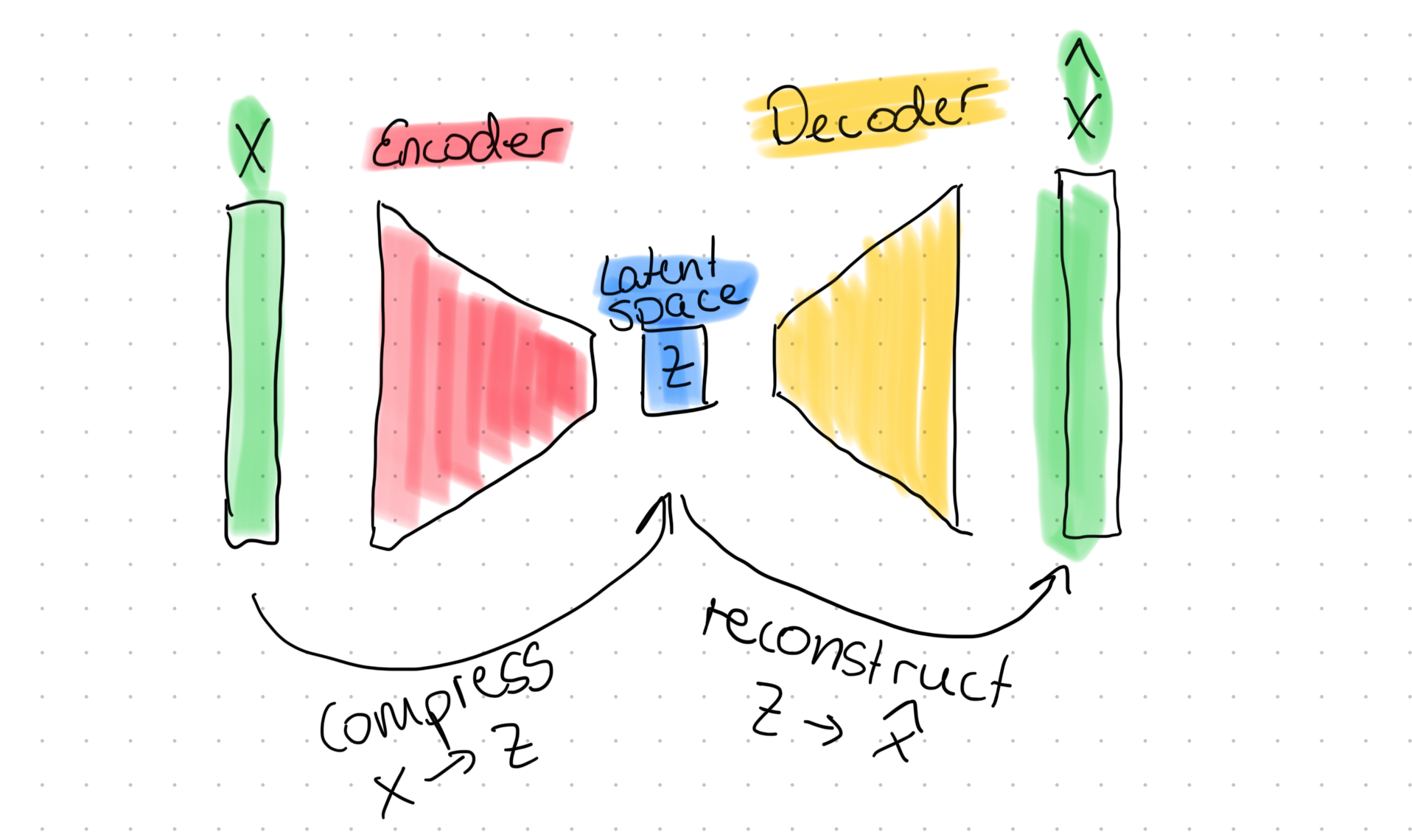
The Variational Autoencoder (VAE) is the successor to the regular autoencoder (AE). As you probably already know, a regular AE is a neural network that compresses its input to a latent space and then reconstructs the orignal input from that latent space. In drawings, you would often find something like this:

This is simple stuff, and you can easily create such a network. Here is a quick example of what an AE looks in code:

class Autoencoder(eqx.Module):
    encoder: eqx.nn.Sequential
    decoder: eqx.nn.Sequential

    def __init__(self, dim: int, hidden_dim: int, z_dim: int, key: PRNGKeyArray):
        key, *subkeys = jax.random.split(key, 10)
        self.encoder = eqx.nn.Sequential(
            [
                eqx.nn.Linear(dim, hidden_dim, key=subkeys[0]),
                eqx.nn.Lambda(fn=jax.nn.relu),
                eqx.nn.Linear(hidden_dim, z_dim, key=subkeys[2]),
            ]
        )

        self.decoder = eqx.nn.Sequential(
            [
                eqx.nn.Linear(z_dim, hidden_dim, key=subkeys[2]),
                eqx.nn.Lambda(fn=jax.nn.relu),
                eqx.nn.Linear(hidden_dim, dim, key=subkeys[2]),
            ]
        )

    def __call__(self, x: Array) -> tuple[Array, Array]:
        z = self.encoder(x)
        o = self.decoder(z)
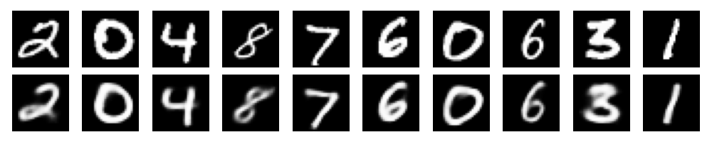
        return o, z

Very simple stuff. Ok, but let’s say you have trained your AE on MNIST and you get get some nice reconstructions like these:

One thing you might be thinking is this: if I give my AE an image of a $1$ and I get some vector $z_1$ back and then I encode an image of a $2$ and get another vector $z_2$ back, then what does the middle point between $z_1$ and $z_2$ look like? After all, I can put either vector $z$ into my decoder and get a nice reconstructed image of my original input back. Does this mean that the middle point between the encoded vectors for the image $1$ and $2$ is an image which looks kind of like both $1$ and $2$? If it wasn’t numbers but faces, can I give the AE 2 faces, take the middle point and put that through the decoder to get a completely new face back?

The unfortunate truth is: no!

But if we could somehow tidy up the latent space, then yes, we could generate new and authentic looking images. And the way we can tidy the latent space up is by using VAE. VAEs solve this by forcing the latent space to follow a specific distribution (Gaussian), which creates a smooth, organized latent space where interpolation works!

In a VAE, we have 2 spaces: the data space $p(x)$ and the latent space $p(z)$ and we don’t really have access to any of those (we only have a bunch of data points sampled from $p(x)$ but that’s about it). VAE has a design decision and says that $p(z)$ is normal distributed and this will be very useful later in the loss function derivation.

Between these, we have 2 mappings (both also normal distributions) that map one space to the other which are:

These mappings are like our encoder and decoder: $p(x|z)$ generates (or reconstructs) $x$ from a latent vector $z$ and vice versa.

And we don’t really know those either (at least so far).

The decoder we can just learn as a supervised learning task and is by far the easiest part: we have the input $z$ and the target $x$ and all we need to do is to compare the output of the decoder against the input $x$ and we’re golden.

But the encoder is a different story, because

which would mean we would have to integrate over the entire latent space $p(z)$, which is computationally not feasible. So, instead, we will approximate $p(z|x)$ with

And we do our training correctly, then $q(z|x)$ will indeed be a good approximation to the true encoder and $q(z|x)$ will also be a normal distribution. And btw. this means that it will output a $\mu$ and a $\sigma$, which we can use to sample the vector $z$.

Deriving the Loss Function

Here’s the goal: we want to maximise $log p(x)$ for each $x$ in our dataset and if you’re asking why, then you’re in good company, because that’s not immediately obvious. Remember how I said we have 2 distributions and that one of them is $p(x)$ - the data distribution? What $log p(x)$ tells us is the probability that we could sample $x$ from the distribution. But all our data points $x$ ARE from the data distribution, so the probability is $1.0$, because we don’t have any datapoints outside of our dataset. So that is our starting point:

The first thing we can say is this:

And that means marginalising out $z$. To better understand this, imagine you had 2 die (an $x$-dice and a $z$-dice) and their probabilities are skewed such that higher numbers have higher probabilities. A probability matrix would look like this:

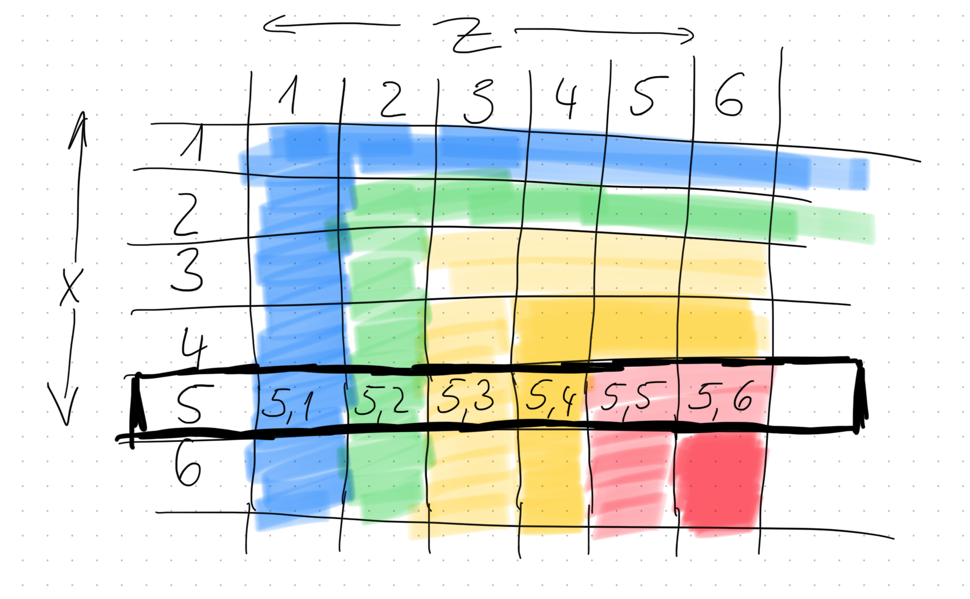
The redder areas indicate a higher probability. If you were interested in the probability that $p(x=5)$, then, to calculate that, you need to compute the sum of all the outcomes where $p(x=5, z=any)$ (that’s the one I highlighted in the image), so, in other words, it’s:

This process is called marginalization. It’s essentially the same as $\log p(x) = \log \int p(x|z) p(z) dz$, except of course there we are dealing with continious values (and the log is there for numerical stability, but doesn’t change the probabilities underneath).

We use the “multiply by one” trick to introduce a new term:

Pretty neat, now we introduced our approximation. We can rearrange some stuff to get this:

The next trick is a bit unintuitive, but bear with me. Let’s say you have two functions:

and another function which generates the $z$ randomly

Think back to the skewed die from earlier. If $Q(z)$ is the random outcome generator for one of those die, then it will return higher values for $z$ with greater probability than lower ones. So what is the expected value for the function $f(z)$ in this case? It is defined as:

Or spoken in plain English: the expected value for the function $f(z)$ is the probability to sample a $z$ times the value of that $z$. For our die example, we could say that we have a 10% change to roll a 1 and a 90% chance to roll a 6 and nothing else. In this case, the expected value for $f(z)$ is

We have the same setting in our derivation:

Where $q(z|x)$ is the probability to sample $z$ (this is akin to the Q(z) from the definition earlier) and $\frac{p(x,z)}{q(z|x)}$ is the value function (the f(z) in the example). With that, we can rewrite it like so:

The next trick we can use is the Jensen inequality, which states:

if $f$ is a concave function and since $\log$ is a concave function, we can say

For our derivation, we can now write:

This is great, because now if we can - somehow - increase $\mathbb{E}_{q(z|x)} \left( \log \frac{p(x,z)}{q(z|x)} \right)$, then it will automatically raise the bar for $\log p(x)$.

Because $p(x,z) = p(x|z)p(z)$, we can write and rearrange the terms like so:

The laws of the logs tell us:

And because of that, we can rewrite the term as:

The blue part trains the decoder, while the green part trains the encoder. Furthermore, the blue part will simplify to the MSE, while the green part is the exact definition of the negative KL divergence. Let’s start with the decoder part, because that’s a bit easier.

I said earlier that the encoder outputs a $\mu$ and a $\sigma$ which we use to sample the latent vector $z$. The decoder technically also outputs both of these, but in practice, we set $\sigma$ to a constant and use $\mu$ directly. Because the decoder is a normal distribution, we can write this:

When it comes to optimization, everything that is a constant, we don’t care about. This means that the only thing that does remain and is NOT constant is:

Which is the mean squared error (and $x_{rec}$ is the output of our decoder). Now, let’s have a look at the encoder:

Which is precisely the definition for the KL divergence, and because $p(z)$ is a normal distribution, the KL divergence simplifies to a closed form:

$\mu_z$ and $\sigma_z$ come from $p(z)$ and because $p(z)$ is a Gaussian, those are $0$ and $1$ respectively and $\mu_e$ and $\sigma_e$ come from $q(z|x)$ (i.e. the encoder approximation).

So, if we put everything together, we get:

The $+\text{const}$ part refers to this part $\frac{d}{2}\log(2\pi)$ which is just some constant and those don’t matter when we minimise in our ML libraries and the same goes for scalars, which is why we dropped the $1/2$ too.

The Code

With the loss function in place, the rest is actually pretty simple. Here is the full code:

import clu.metrics as clum
import equinox as eqx
import jax
import jax.numpy as jnp
import matplotlib.pyplot as plt
import numpy as np
import optax
import tensorflow as tf
import tensorflow_datasets as tfds
from jaxtyping import Array, Float, PRNGKeyArray, PyTree
from tqdm import tqdm


class LossMetrics(eqx.Module, clum.Collection):
    loss: clum.Average.from_output("loss")  # pyright: ignore


tf.random.set_seed(42)
np.random.seed(42)

(train_ds, test_ds), ds_info = tfds.load(
    "mnist",
    split=["train", "test"],
    shuffle_files=True,
    as_supervised=True,
    with_info=True,
)  # pyright: ignore


def preprocess(image, label):
    image = tf.cast(image, tf.float32) / 255.0
    image = tf.reshape(image, (-1,))
    return image, label


BATCH_SIZE = 128

train_ds = train_ds.map(preprocess)
train_ds = train_ds.cache()
train_ds = train_ds.shuffle(ds_info.splits["train"].num_examples)
train_ds = train_ds.batch(BATCH_SIZE)
train_ds = train_ds.prefetch(tf.data.AUTOTUNE)

test_ds = test_ds.map(preprocess)
test_ds = test_ds.batch(BATCH_SIZE)
test_ds = test_ds.prefetch(tf.data.AUTOTUNE)


def reparameterize(mu: Array, logvar: Array, key: PRNGKeyArray) -> Array:
    std = jnp.exp(0.5 * logvar)
    eps = jax.random.normal(key, shape=mu.shape)
    return mu + std * eps


class Encoder(eqx.Module):
    layers: eqx.nn.Sequential

    mu_layer: eqx.nn.Linear
    logvar_layer: eqx.nn.Linear

    def __init__(
        self, input_dim: int, hidden_dim: int, latent_dim: int, key: PRNGKeyArray
    ):
        key, *subkeys = jax.random.split(key, 10)

        self.layers = eqx.nn.Sequential(
            [
                eqx.nn.Linear(input_dim, hidden_dim, key=subkeys[0]),
                eqx.nn.Lambda(jax.nn.relu),
                eqx.nn.Linear(hidden_dim, hidden_dim, key=subkeys[1]),
                eqx.nn.Lambda(jax.nn.relu),
            ]
        )

        self.mu_layer = eqx.nn.Linear(hidden_dim, latent_dim, key=subkeys[2])
        self.logvar_layer = eqx.nn.Linear(hidden_dim, latent_dim, key=subkeys[3])

    def __call__(self, x: Float[Array, " input_dim"]) -> tuple[Array, Array]:
        x = self.layers(x)
        mu = self.mu_layer(x)
        logvar = self.logvar_layer(x)

        return mu, logvar


class Decoder(eqx.Module):
    layers: eqx.nn.Sequential

    def __init__(
        self, latent_dim: int, hidden_dim: int, output_dim: int, key: PRNGKeyArray
    ):
        key, *subkeys = jax.random.split(key, 10)

        self.layers = eqx.nn.Sequential(
            [
                eqx.nn.Linear(latent_dim, hidden_dim, key=subkeys[0]),
                eqx.nn.Lambda(jax.nn.relu),
                eqx.nn.Linear(hidden_dim, hidden_dim, key=subkeys[1]),
                eqx.nn.Lambda(jax.nn.relu),
                eqx.nn.Linear(hidden_dim, output_dim, key=subkeys[2]),
            ]
        )

    def __call__(self, z: Float[Array, "latent_dim"]) -> Array:
        x = self.layers(z)
        return x


class VAE(eqx.Module):
    encoder: Encoder
    decoder: Decoder

    def __init__(
        self, input_dim: int, hidden_dim: int, latent_dim: int, key: PRNGKeyArray
    ):
        key, *subkeys = jax.random.split(key, 5)
        self.encoder = Encoder(input_dim, hidden_dim, latent_dim, key=subkeys[0])
        self.decoder = Decoder(latent_dim, hidden_dim, input_dim, key=subkeys[1])

    def __call__(self, x: Array, key: PRNGKeyArray):
        mu, logvar = self.encoder(x)
        z = reparameterize(mu, logvar, key)

        reconstructed_x = self.decoder(z)
        return reconstructed_x, mu, logvar


def vae_loss(
    model: VAE, x: Float[Array, "batch_size input_dim"], key: PRNGKeyArray
) -> Array:
    keys = jax.random.split(key, len(x))
    reconstructed_x, mu, logvar = eqx.filter_vmap(model)(x, keys)

    recon_loss = jnp.mean(jnp.sum(jnp.square(x - reconstructed_x), axis=-1))

    kl_loss = -0.5 * jnp.mean(
        jnp.sum(1 + logvar - jnp.square(mu) - jnp.exp(logvar), axis=-1)
    )

    total_loss = recon_loss + kl_loss
    return total_loss


vae_model = VAE(input_dim=784, hidden_dim=128, latent_dim=8, key=jax.random.key(44))

images, labels = next(iter(train_ds.take(1)))
images = jnp.array(images)
labels = jnp.array(labels)
loss = vae_loss(vae_model, images, key=jax.random.key(42))
print(loss)

learning_rate = 3e-4
optimizer = optax.adam(learning_rate)
opt_state = optimizer.init(eqx.filter(vae_model, eqx.is_array))


@eqx.filter_jit
def step(
    model: PyTree,
    x: Array,
    optimizer: optax.GradientTransformation,
    opt_state: optax.OptState,
    key: PRNGKeyArray,
):
    loss, grads = eqx.filter_value_and_grad(vae_loss)(model, x, key)
    updates, opt_state = optimizer.update(grads, opt_state, model)
    model = eqx.apply_updates(model, updates)

    return loss, model, opt_state


n_epochs = 500

metrics = LossMetrics.empty()
key = jax.random.key(0)
for epoch in tqdm(range(n_epochs)):
    for images, _ in train_ds:
        images = jnp.array(images)
        key, subkey = jax.random.split(key)
        loss, vae_model, opt_state = step(
            vae_model, images, optimizer, opt_state, subkey
        )
        metrics = metrics.merge(LossMetrics.single_from_model_output(loss=loss))

    print(f"Epoch {epoch}, loss {metrics.compute()}")


eqx.tree_serialise_leaves("mnist_vae", vae_model)

vae_model = eqx.tree_deserialise_leaves("mnist_vae", vae_model)


def visualize_reconstructions(model, images, n=10):
    # Get the first n images
    original = images[:n]

    # Reconstruct images
    key = jax.random.key(0)
    keys = jax.random.split(key, n)
    reconstructed, _, _ = eqx.filter_vmap(model)(original, keys)

    # Reshape for visualization
    original = original.reshape(-1, 28, 28)
    reconstructed = reconstructed.reshape(-1, 28, 28)

    # Plot
    fig, axes = plt.subplots(2, n, figsize=(n, 2))
    for i in range(n):
        axes[0, i].imshow(original[i], cmap="gray")
        axes[0, i].axis("off")
        axes[1, i].imshow(reconstructed[i], cmap="gray")
        axes[1, i].axis("off")

    plt.tight_layout()
    plt.savefig("reconstructions.png")
    plt.close()


# Generate random samples from the latent space
def visualize_samples(model, n=10):
    # Sample from the latent space
    key = jax.random.key(42)
    z = jax.random.normal(key, shape=(n, model.encoder.mu_layer.out_features))

    # Decode the samples
    samples = eqx.filter_vmap(model.decoder)(z)

    # Reshape for visualization
    samples = samples.reshape(-1, 28, 28)

    # Plot
    fig, axes = plt.subplots(1, n, figsize=(n, 1))
    for i in range(n):
        axes[i].imshow(samples[i], cmap="gray")
        axes[i].axis("off")

    plt.tight_layout()
    plt.savefig("samples.png")
    plt.close()


# Call these after training
test_images, _ = next(iter(test_ds))
test_images = jnp.array(test_images)
visualize_reconstructions(vae_model, test_images)
visualize_samples(vae_model)

If you run this code, you will get this neat images:

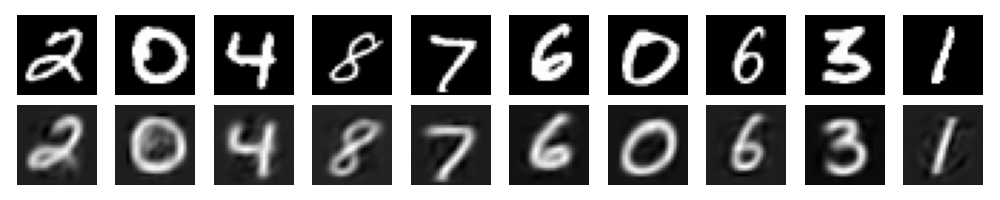
These are the reconstructions from the VAE. You can compare those to the reconstructions from the normal AE:

And now the real kicker, which are the newly generated samples:

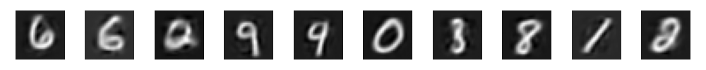
One thing that needs more context is this function:

def reparameterize(mu: Array, logvar: Array, key: PRNGKeyArray) -> Array:
    std = jnp.exp(0.5 * logvar)
    eps = jax.random.normal(key, shape=mu.shape)
    return mu + std * eps

And why we use this function in the VAE class instead of directly sampling using mu and logvar from the encoder, which would look like this:

np.random.normal(loc=mu, scale=logvar, size=10) # in Numpy

Well, for one, we can’t even pass the mean and variance to the jax.random.normal function, and even if we could, what is the gradient in that case? Well, there is no gradient; it would be interrupted. That’s why we use this reparameterize-trick instead.